Implementing the Path Tracer

What have we learned

• Today we will finally implement our path tracer, which concludes the discussion on the rendering equation

• Even though there are still two weeks until the end of the course, we can already evaluate what we should have learned from the course

• Let’s do it with a question…

What bugs do you expect today?

Work Methodology

• We have always implemented one feature at a time (saving images, tone mapping, projections…)

• For each feature, we implemented a series of tests

• This is why every week we had the confidence that when we relied on code written in previous weeks, it was probably “correct”

• It is impossible to write code as long as the one you produced so far without proceeding this way

• This is the most important lesson provided by this course!

Orthonormal Bases (ONB)

Creating ONBs

• It is convenient to use the algorithm from Duff et al. 2017:

  def create_onb_from_z(normal: Union[Vec, Normal]) -> Tuple[Vec, Vec, Vec]:
      # In Python there isn't a `copysign` function 🙁
      sign = 1.0 if (normal.z > 0.0) else -1.0
      a = -1.0 / (sign + normal.z)
      b = normal.x * normal.y * a
  
      e1 = Vec(1.0 + sign * normal.x * normal.x * a, sign * b, -sign * normal.x)
      e2 = Vec(b, sign + normal.y * normal.y * a, -normal.y)
  
      return e1, e2, Vec(normal.x, normal.y, normal.z)

• When calling this function, pay close attention to the fact that the normal parameter must already be normalized!

Testing

• To verify the correct operation of create_onb_from_z, we can use random testing (an idea apparently originating in the world of the Haskell language, see quickcheck).

• The idea is to generate a large number of random vectors, pass them as parameters to create_onb_from_z, and verify that the return type is indeed an ONB. (Apparently Duff et al. discovered the bug in the algorithm from Frisvad, 2012 this way).

• The general approach of random testing is to generate random inputs and verify that the outputs satisfy certain properties. It is especially convenient for mathematical functions, but it is not always the best solution.

Random testing in pytracer

pcg = PCG()  # Use the default seed, so if the test fails you can debug it
expected_zero, expected_one = pytest.approx(0.0), pytest.approx(1.0)

# As Python is slow, we just test 100 times the function. You can use
# larger numbers, as far as the time required to run the test is kept short
for i in range(100):
    # We could use a fancier code that samples uniformly over the 4π sphere…
    normal = Vec(*[pcg.random_float() for i in range(3)]).normalize()
    e1, e2, e3 = create_onb_from_z(normal)

    # Verify that the z axis is aligned with the normal
    assert e3.is_close(normal)

    # Verify that the base is orthogonal
    assert expected_zero == e1.dot(e2)
    assert expected_zero == e2.dot(e3)
    assert expected_zero == e3.dot(e1)

    # Verify that each component is normalized
    assert expected_one == e1.squared_norm()
    assert expected_one == e2.squared_norm()
    assert expected_one == e3.squared_norm()

    # You could also check that e₁×e₂=e₃, e₂×e₃=e₁, e₃×e₁=e₂

Importance sampling

Implementation

• We anticipated that our path tracer will use the Monte Carlo method to estimate the integral of the rendering equation:

  \int_{2\pi} f_r(x, \Psi \rightarrow \Theta)\,L(x \leftarrow \Psi)\,\cos\theta\,\mathrm{d}\omega_\Psi.

• To improve variance we will use importance sampling, employing the PDF

  p(\omega) \propto f_r \cdot \cos\theta.

The BRDF Type

• We therefore need to add a method that applies to the types derived from BRDF and that has this signature:

  def scatter_ray(self,
      pcg: PCG,                    # Used to generate random numbers
      incoming_dir: Vec,           # Direction of the incoming ray
      interaction_point: Point,    # Where the ray hit the surface
      normal: Normal,              # Normal on interaction_point
      depth: int,                  # Depth value for the new ray
  ) -> Ray

• Each type derived from BRDF (e.g., DiffuseBRDF, SpecularBRDF, etc.) will have to redefine scatter_ray.

DiffuseBRDF

• For the diffuse BRDF, we deduced that p(\omega) \propto \cos\theta.

• The implementation of DiffuseBRDF.scatter_ray must therefore use the algorithm we derived for the Phong distribution with n = 1:

  def scatter_ray(self, pcg: PCG, incoming_dir: Vec,
                  interaction_point: Point, normal: Normal, depth: int) -> Ray:
      e1, e2, e3 = create_onb_from_z(normal)
      cos_theta_sq = pcg.random_float()
      cos_theta, sin_theta = sqrt(cos_theta_sq), sqrt(1.0 - cos_theta_sq)
      phi = 2.0 * pi * pcg.random_float()
  
      return Ray(origin=interaction_point,
                 dir=e1 * cos(phi) * cos_theta + e2 * sin(phi) * cos_theta + e3 * sin_theta,
                 tmin=1.0e-3,   # Be generous here
                 tmax=inf,
                 depth=depth)

SpecularBRDF

• Ray generation for the specular BRDF is perfectly deterministic, and there is no \cos\theta term to weight the ray’s contribution.

• The implementation of SpecularBRDF.scatter_ray is therefore particularly simple:

  def scatter_ray(self, pcg: PCG, incoming_dir: Vec,
                  interaction_point: Point, normal: Normal, depth: int) -> Ray:
      ray_dir = Vec(incoming_dir.x, incoming_dir.y, incoming_dir.z).normalize()
      normal = normal.to_vec().normalize()
  
      return Ray(origin=interaction_point,
                 dir=ray_dir - normal * 2 * normal.dot(ray_dir),
                 tmin=1e-3,
                 tmax=inf,
                 depth=depth)

Path tracing

The PathTracer Type

• We have defined two renderers so far: OnOffRenderer and FlatRenderer. Today we implement PathTracer.

• The constructor parameters are as follows:

  1. The World object to render;
  2. The background color, used for those directions along which there are no intersections;
  3. The random number generator to use (PCG type);
  4. Number of rays to generate for the integral calculation;
  5. Maximum ray depth;
  6. Depth limit beyond which to use Russian Roulette.

Implementation

def __call__(self, ray: Ray) -> Color:
    return Color(0.0, 0.0, 0.0) if ray.depth > self.max_depth

    hit_record = self.world.ray_intersection(ray)
    return self.background_color if not hit_record

    hit_material = hit_record.material
    hit_color = hit_material.brdf.pigment.get_color(hit_record.surface_point)
    emitted_radiance = hit_material.emitted_radiance.get_color(hit_record.surface_point)

    hit_color_lum = max(hit_color.r, hit_color.g, hit_color.b)

    if ray.depth >= self.russian_roulette_limit:  # Russian roulette
        q = max(0.05, 1 - hit_color_lum)
        if self.pcg.random_float() > q:
            # Keep the recursion going, but compensate for other potentially discarded rays
            hit_color *= 1.0 / (1.0 - q)
        else:
            # Terminate prematurely
            return emitted_radiance

    # Monte Carlo integration

    cum_radiance = Color(0.0, 0.0, 0.0)

    # Only do costly recursions if it's worth it
    if hit_color_lum > 0.0:
        for ray_index in range(self.num_of_rays):
            new_ray = hit_material.brdf.scatter_ray(
                pcg=self.pcg,
                incoming_dir=hit_record.ray.dir,
                interaction_point=hit_record.world_point,
                normal=hit_record.normal,
                depth=ray.depth + 1,
            )
            new_radiance = self(new_ray)  # Recursive call
            cum_radiance += hit_color * new_radiance

    return emitted_radiance + cum_radiance * (1.0 / self.num_of_rays)

Test

• A simple method to verify the functioning of a path tracer is the so-called furnace test.

• It consists of casting a ray inside an arbitrarily shaped object with diffuse BRDF and constant luminosity L_e and reflectance \rho_d.

• The generic ray will follow a path trapped within the object, and thus each ray will keep hitting the same sphere over and over again. This is a situation where the rendering equation can be solved analytically.

\begin{aligned} L &= L_e + \rho_d \Bigl(L_e + \rho_d \bigl(L_e + \rho_d(L_e + \dots)\bigr)\Bigr) =\\ &= L_e + \rho_d L_e + \rho_d^2 L_e + \rho_d^3 L_e + \ldots =\\ &= L_e \bigl(1 + \rho_d + \rho_d^2 + \rho_d^3 + \ldots \bigr) =\\ &= L_e \sum_{n=0}^\infty \rho_d^n =\\ &= \frac{L_e}{1 - \rho_d}. \end{aligned}

Tests in Pytracer

• The pytracer code implements the test testFurnace which uses these assumptions:

  1. Creates a sphere centered at the origin;
  2. Casts a ray starting from the center of the sphere;
  3. Invokes PathTracer setting max_depth=100 and ensuring that the Russian roulette algorithm is not used;
  4. Verifies that the returned radiance corresponds to L_e / (1 - \rho_d).

• The test is repeated a number of times using random values of L_e and \rho_d (avoiding choosing \rho_d \approx 1!).

The main Method

• Now that we have a path tracer, it’s good to modify our demo command so that it creates an image that better highlights how the algorithm works.

• You can define any scene you like, using the shapes you have implemented in your code (spheres, planes, triangles, CSG, etc.).

• The important thing is that you define a large diffuse surface (a plane or a large radius sphere), which acts as a light source and therefore has a non-negligible L_e component.

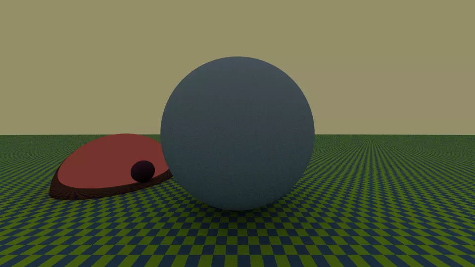
• In pytracer I defined a plane for the ground, a sphere for the sky, and two spheres in the foreground: the first has a diffuse BRDF, the second a reflective BRDF.

Random Numbers

• Make sure that the two numbers that initialize the PCG generator can be passed from the command line.

• The most important number is init_seq, because it uniquely identifies the sequence of numbers generated by the PCG, and therefore allows the production of completely decorrelated images (which can then be averaged together without producing bias).

• Averaging different images (produced concurrently using GNU Parallel) is a good way to reduce variance without increasing the actual computation time (wall-clock time).

Profiling

Profiling

• From today, your code will have to do a lot of calculations!

• Compare the code speeds of different groups in generating similar images, to understand if there are bottlenecks: with the languages you use, in theory there shouldn’t be significant differences.

• If you notice differences, you need to measure which part of the code is slowing it down: this is what is called profiling.

Performance Measurement

• It is not enough to know how long your entire code takes to produce an image: you need to know how much time it spends in each function.

• There are various ways to measure it, and many tools available: it’s impossible to be exhaustive!

• I’ll list some possibilities, and offer some tips and tricks.

Types of Profilers

• The simplest method is to surround the functions «suspected» of being bottlenecks with time measurements:

  from time import perf_counter_ns   # Or: "monotonic". DO NOT USE ANYTHING ELSE!!
  start = perf_counter_ns()
  long_function_call(...)
  elapsed_time = perf_counter_ns() - start

• There are profilers that measure the cumulative time spent by each line of code: be careful, because they can slow down the code a lot!

• Statistical profilers are also available, which are less accurate but do not significantly slow down the code.

Outsmarting the compiler

• Modern compilers are so smart that they can make benchmark results worthless.

• For instance, the following code will likely report that the cross product of two vectors takes no time to run:

  Vec a{1.0, 2.0, 3.0}, b{5.0, 4.0, 2.0}, c;
  auto time0{perf_conter()};
  const int N{10'000'000};
  for(int i{}; i < N; ++i) {
      c = cross(a, b);
  }
  auto time1{perf_counter()};
  println("Time: {}" (time1 - time0) / N);  // This is likely zero!

Tips (1/4)

• Never test mathematical functions on variables set to zero, as compilers usually optimize these calls out

• If you initialize your variables to random numbers, be sure not to include random number generator in the profiling! Good practice: initialize a vector of random numbers before the test:

  vector inputs{100'000};
  for(int i{}; i < ssize(inputs); ++i) {
      inputs[i] = gen_random();
  }
  
  // Now run the benchmark
  auto time0{perf_conter()};
  // etc.

Tips (2/4)

• Other stuff might happen while your benchmark code is running:

  1. If you are using a Just-in-time (JIT) compiler (Julia, C#, Java, etc.), the first time you call a function it needs to be compiled/optimized
  2. Your language might perform garbage collection (C#, Julia, Go, D, etc.);
  3. Your system might dynamically adjust CPU frequency to optimize power drain;
  4. Other processes (OS updater, email client) might run in the background;
  5. Etc.

• It might be that you are measuring the time spent to run your program and to do something else.

Tips (3/4)

• It’s a good idea to run a benchmark a few times (3? 5?) and then consider the minimum time alongside other statistical parameters (average, median, etc.).

• Many benchmark libraries provide detailed statistics and consider JIT warm-up times and other nuisances: Google Benchmark (C++), BenchmarkTools.jl (Julia), BenchmarkDotNet (C#, F#), etc.

Tips (4/4)

• Don’t measure the time of every function, just focus on the ones that could be problematic. (For example, it doesn’t matter if the function that interprets the command line is fast!)

• Often the output of profilers is quite unreadable and too detailed: however, there are tools to extract summary graphs such as flamegraphs, which are easier to read.

• The speedscope site provides a way to produce navigable flamegraphs through a browser, starting from the output of various profilers, and does not require installation.

What to do today

What to do today

1. Continue working in the pathtracing branch;
2. Implement a function to create an orthonormal basis starting from a normal vector (if in your language it is not easy to return three return values, implement a new ONB type);
3. Implement the scatter_ray method that works on BRDF types, and implement the specular BRDF;
4. Implement the path tracing algorithm;
5. Modify the demo so that it has a diffuse sky capable of illuminating the scene.
6. After merging, release version 0.3.0 and update the CHANGELOG.md file.

Optional Additions

• Antialiasing (see PR#13 of pytracer);
• Point-light tracing (see PR#14 of pytracer).