Laboratory 10
Calcolo numerico per la generazione di immagini fotorealistiche
Maurizio Tomasi maurizio.tomasi@unimi.it
Generating pseudorandom numbers
Pseudorandom numbers
You have surely already dealt with random numbers, probably to perform Monte Carlo simulations (see e.g. the TNDS course).
In this course we will not address the problem of random number generation in detail, but we will use a series of results without proving them.
The context of photorealistic images is interesting to verify the operation of a random number generator: if the quality of the generator is not excellent, you spot it immediately!

How a generator works
A pseudorandom number generator is usually implemented as a state machine, i.e., an algorithm that keeps information about its state in memory, which is updated every time it produces a new number.
The generators used today usually produce integer numbers in a given range.
Being only pseudo-random, if you know the last number drawn and the state of a generator, you can predict what the next number will be (determinism). This can be an advantage!
Quality of a generator
The numbers it produces should be “random” (see the Wikipedia entry Randomness test)…
…but also predictable!
Numbers taken in pairs/triples/quadruples/etc. should continue to be “random”.
It should be fast to execute.
It should be possible to quickly advance its internal state: this property is called seekability.
1. “Randomness”
A deterministic pseudo-random number generator must have a certain period N: once N values have been extracted, it is doomed to repeat the sequence again (or, in rare cases, to stop).
It is important that the first N values are distributed as uniformly as possible.
It is also important that the period is sufficiently long!
(In the study of the PICO satellite we had encountered strange results, due to the fact that the period of the generator was “only” 2^{32} and therefore after a certain time the code reviewed the same numbers from the beginning.)
2. Predictability
Since pseudo-random numbers are used for computer simulations, it is important to be able to debug the code.
If the generator’s numbers were truly random and we encountered a problem that only emerges from time to time, debugging would be very difficult!
Usually generators require to be initialized with a “seed”: if you provide the same seed twice, the sequence of numbers is the same.
This can be extremely useful!
3. Dimensionality
Random numbers are often used to produce random vectors, i.e., samples x \in \mathbb{R}^n, for some value of n (for example, points on the plane with n = 2, points in space with n = 3, etc.).
A bad random number generator can work perfectly in generating 1D sequences, but show strange correlations when used to generate 2D points.
A generator that maintains the properties of “randomness” in k dimensions is said to satisfy k-dimensional equidistribution.
Example
Suppose that a generator produces 32-bit numbers where the first 31 bits are “random”, but the last bit regularly alternates between 0 and 1:
- 11101111011000101101011101110010 (even number)
- 10100010101001000010000101110101 (odd number)
- 01000011011001011001111110001110 (even number)
- 01010110110011101010001101010111 (odd number)
- Etc., so that all values between 0 and 2³²−1 are extracted once
If I want to produce random 2D points (x, y) uniformly distributed, the abscissas will always have an even value and the ordinates an odd value ⇒ half of the theoretically possible points will actually never be chosen!
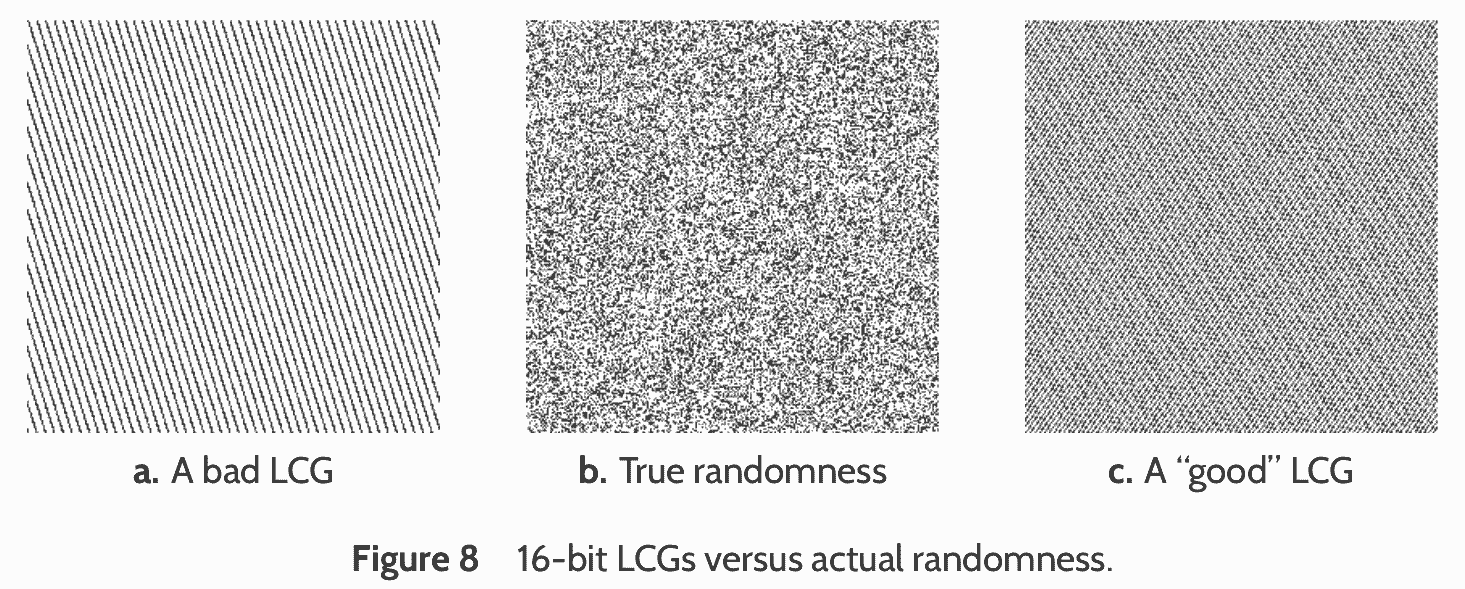
A randogram (see O’Neill, 2014).
4. Performance
Applications of Monte Carlo methods to physics require running many simulations to reduce the effects of sampling.
One way to achieve high speed is to use bitwise logical operations, which are the fastest operations that can be performed on common CPUs.
A generator should keep its state in the smallest possible memory structure: this makes it easier for the CPU to optimize its execution.
5. Seekability
In a generator, each random number is derived from the generator’s state, and the state changes for each new number generated. Consequently, the random value x_{k + 1} depends on the knowledge of the value x_k.
If I wanted to produce 2\times 10^9 random numbers using two computers, I might want to generate 10^9 samples on the first machine and 10^9 on the second.
However, if the problem is not set up correctly, there is a risk that the two sample sequences will be correlated.
Example
If I assign the same seed to the two computers, I get the same sequence: argh!
I could then assign the seed 5 to the first computer and the seed 36 to the second.
However, if the generator is such that after the number 5 it extracts the number 36, the sequence of generated numbers is then the following:
computer #1:  5  36  17  29  45  …
computer #2: 36  17  29  45   3  …
Obviously, this would also be a problem if I assigned 17, 29, or 45 to the second computer instead of 36.
It is not enough to give a different seed to the two computers to obtain independent sequences!
Solutions to the problem
One possible solution is to have a criterion whereby two states of the generator are orthogonal: that is, they cannot generate the same sequence of samples, not even shifted. These generators typically require initialization with two initial numbers: a sequence identifier and the seed. If two different identifiers are used, the generated sequences are uncorrelated.
Another solution is to be able to advance the state of the generator by k steps quickly, without actually generating k - 1 random numbers and requiring a number of operations much less than \sim k (typically \sim \log k).
Parallel Generation
To generate a long sequence of N random numbers by distributing it over k computers, the following procedure can be used:
Start with a fixed seed, or a random one (obtained from the date and time the program was executed), and create the initial state of the generator;
Assign to each of the k computers the task of generating only N/k samples, and copy the same initial state of the generator to each of them;
On the i-th computer, advance the generator state by i \times N / k, using the “fast” algorithm;
Each generator proceeds to generate the N/k samples.
Algorithms
The standard libraries of compilers offer functionality for generating random numbers, but the quality of these generators is very uneven!
In 2014, Melissa O’Neill published a fantastic article on a new family of random number generators that satisfies all the characteristics listed above, and it is released as an open-source library on the website www.pcg-random.org.
In this course, we will therefore use the PCG algorithm, which has all the nice properties listed above.
The PCG Algorithm
The algorithm we will implement to generate pseudo-random numbers is described in the same article O’Neill (2014).
Even if there might be PCG implementations in your language, you are required to implement it yourself.
There are in fact numerous variants of the algorithm, which are distinguished by the bit size of the quantities used during generation.
If everyone uses the same generator with the same seed, it will be easier to do cross-group debugging!
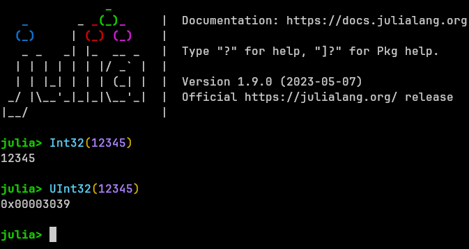
Unsigned Numbers
PCG, like many similar algorithms, requires calculations with bit masks.
Bit masks are usually encoded with unsigned integers.
![]()
A negative number like
-12(0b1100) is encoded with two’s complement: all bits of12are inverted and 1 is added, resulting in0b11110100(8 bits).
Bitwise Operations
| Name | Example (Julia) |
|---|---|
| And | 0b1001 & 0b0011 == 0b0001 |
| Or | 0b1001 | 0b0011 == 0b1011 |
| Xor | 0b1001 ^ 0b0011 == 0b1010 |
| Arithmetic shift | 0b1001 >> 1 == 0b100 |
Int8(-12) >> 1 == -6 |
|
Int16(-12) >> 1 == -6 |
|
| Logical shift | 0b1001 >>> 1 == 0b100 |
Int8(-12) >>> 1 == 122 |
|
Int16(-12) >>> 1 == 32762 |
In a right arithmetic shift, the new most significant bit is a copy of the old one, so as to preserve the sign. (See this article.)
In a logical shift, the new most significant bit is always zero, and this is the one to use in PCG.
Implementation in Python
The PCG algorithm requires wrapping when integers overflow. Many languages (C++, C#, Julia…) satisfy this requirement for unsigned types.
However, in Python there is only one
inttype, whose size adapts depending on the number to be stored.Overflows are not possible in Python because the Python interpreter always allocates more space to avoid losing digits.
The languages you use, on the other hand, optimize for performance and can experience overflows. These overflows are not only accepted, but actually required in the PCG algorithm.
Integer Management
To make Python behave more like Julia, I had to implement a function that masks the least significant bits, simulating 64-bit and 32-bit numbers.
Here is an example
Obviously, this is not necessary when using languages that implement fixed-size integer types. This is the case with all the languages you are using 😀.
Integers Used by PCG
The PCG algorithm we will implement is the one that generates 32-bit numbers in the range [0, 2^{32} - 1] (
uint32_tin C++).The data structure used by the PCG algorithm needs to store two 64-bit
unsignedintegers internally.Familiarize yourselves with the unsigned integer types provided by your language. (Languages like Java don’t have unsigned integers, so you have to make do with signed ones 🙁; however, Kotlin implements them 🥳)
I wrote a blog post about the caveats when working with unsigned types: Use of
unsigned intin C++. Even if you do not use C++, it might be worth reading it.
PCG in Python
Here is the implementation of the
PCGtype and the constructor:@dataclass class PCG: state: int = 0 # 64-bit unsigned integer inc: int = 0 # 64-bit unsigned integer def __init__(self, init_state=42, init_seq=54): self.state = 0 self.inc = (init_seq << 1) | 1 self.random() # Throw a random number and discard it self.state += init_state self.random() # Throw a random number and discard itIn Python, we cannot specify the bits we need, but in your implementations, you will have to declare
stateandincas 64-bitunsignedintegers.
The PCG.random Method
def random(self) -> int:  # 32-bit unsigned number (in Java, return a 64-bit number)
    oldstate = self.state    # 64-bit unsigned integer

    self.state = to_uint64((oldstate * 6364136223846793005 + self.inc))

    # "^" is the xor operation
    xorshifted = to_uint32((((oldstate >> 18) ^ oldstate) >> 27))

    # 32-bit variable
    rot = oldstate >> 59

    # Rotation with a wrap
    return to_uint32((xorshifted >> rot) | (xorshifted << ((-rot) & 31)))
Wrapped rotation
This Python code implements a “wrapped rotation” of the bits:
Check what your language offers to implement this operation effectively:
- In C++20 you can use
std::rotr(in<bit>); - In Rust, there is
xorshifted.rotate_right(rot); - In Java/Kotlin, use
Integer.rotateRight(xorshifted, rot).
- In C++20 you can use
Remember that you need a 32-bit value; depending on your language, you might have to apply a two’s complement (
& 0xffffffffL).
Tests for PCG
def test_random():
    pcg = PCG()

    # You can check these members in a test only if you
    # did not declare "state" and "inc" as private members
    # of the PCG type
    assert pcg.state == 1753877967969059832
    assert pcg.inc == 109

    for expected in [2707161783, 2068313097,
                     3122475824, 2211639955,
                     3215226955, 3421331566]:
        assert expected == pcg.random()
Floating-Point Numbers
Obviously, the
PCG.randommethod returns an integer.In path tracing, however, we will always need pseudo-random numbers X_i uniformly distributed on [0, 1) (avoiding 1 helps when computing quantities that are ill-behaved near x=1, like
acos(1 - x)).Since the PCG implementation returns 32-bit numbers, it is sufficient to normalize the integers returned by the algorithm with 2^{32} to obtain the uniform distribution on [0, 1):
Seed
Make sure that the constructor of the
PCGtype accepts the following default parameters:init_state = 42 init_seq = 54This way, in the tests, it will be enough to create a
PCGvariable with the default constructor, and the test will be repeatable (and comparable between different groups!).
BRDFs
Data Types
Today we will start implementing our path-tracer, and we will begin with materials, BRDFs, and pigments. We will need these primitive data types:
- The
Pigmenttype is abstract and represents the color associated with a particular point on a surface (u, v); - The
BRDFtype is abstract and represents the BRDF of a material, which must contain aPigmentmember; - The
Materialtype is concrete and represents the union of the emissive part of a material (the L_e term, still aPigment) and its BRDF.
- The
From the abstract types
PigmentandBRDF, we will then derive a series of concrete types.
Pigment
The base type
Pigmentis used to calculate a color (typeColor) associated with a coordinate (u, v), through a method/functionget_color, which associates aVec2Dwith aColor.You should at least define these two types:
UniformPigment(uniform color, the simplest pigment!);CheckeredPigment(checkerboard, useful for debugging).
You could also define an
ImagePigmentthat is constructed from anHdrImage: this allows creating very interesting effects if applied to spheres with images containing equirectangular projections. Use the implementation in pytracer as a reference.
Checkered Pigment

Color 1 is used in the squares where the row and column numbers are both even or odd, color 2 in the other cases. The number of divisions should be configurable in the constructor.
BRDF
The
BRDFtype must encode the BRDF of the rendering equation, i.e.,f_r = f_r(x, \Psi \rightarrow \Theta).
The BRDF is by definition a scalar, but to represent the dependence on the wavelength \lambda, the Python code returns a
Colorinstead of afloat: each component (R/G/B) is the BRDF integrated over that band.This is the prototype of
BRDF.Evalas implemented in pytracer:
BRDF and Pigment
The
BRDFtype should contain aPigmenttype or a derivative (in C++ for example, a pointer would be used, orstd::shared_ptr<Pigment>).Use the R/G/B components returned by the pigment for a given point (u, v) on the surface to “weight” the contribution of f_r to the various frequencies (if one of the RGB components is zero, all photons in that band are absorbed).
This is, for example, the implementation of the diffuse BRDF (f_r = \rho_d / \pi) in pytracer, which effectively assumes \rho_d = \rho_d(\lambda):
Material
The
Materialtype must encompass the information about the interaction between surface points and photons:- The BRDF f_r = f_r(x, \Psi \rightarrow \Theta);
- The emitted radiance as a function of the point on the surface: L_e = L_e(u, v).
In pytracer it is defined as follows:
Versatility
The
Pigmenttype only needs to return a color given a coordinate (u, v), so it only requires aget_colormethod. (It could therefore be rethought as a function object, if desired…)The
BRDFtype will have to become more complex than how we implemented it today (in a path tracer, it is not necessary to evaluate f_r, and therefore we will useBRDF.evalfor other purposes!), so it is better not to use shortcuts.The
Materialtype is simply the union of a BRDF and a pigment (the L_e term), and will not be extended.
Updating Shape
You must add an instance of a
MaterialinsideShape:The
HitRecordtype should be modified to also contain a pointer to theShapeobject that was “hit” by the ray: this way it will be possible to trace back to theMaterialto use during the resolution of the rendering equation (an alternative is to saveMaterialinstead ofShape).
Flat-renderer
Now that we have assigned a
Materialto eachShape, it is possible to create a slightly more interesting renderer than the on/off type used in our demo.Specifically, we could implement a simple renderer that, instead of using black and white colors, assigns to a pixel the color of the
Pigmentcalculated at the point where the ray hits the object.The pytracer code implements a base class,
Renderer, from which two classes derive:OnOffRendererandFlatRenderer: when running thedemocommand, you can choose which one to use via the--algorithmflag.
(Due to the image being almost completely black, the tone mapping saturates the colors if the standard brightness value is used; convert the image by setting an average brightness of ~0.5).
Generating Animations
Generating a long animation can be very tedious.
If your computer’s CPU supports multiple cores (very likely), you can use GNU Parallel (
sudo apt install parallelunder Debian/Ubuntu/Mint) to use all cores and produce many frames simultaneously: the time savings are impressive!Write a script
generate-image.shthat produces an image given a numeric parameter and make it executable withchmod +x FILENAME, then run theparallelcommand in a way similar to this:parallel -j NUM_OF_CORES ./generate-image.sh '{}' ::: $(seq 0 359)
generate-image.sh
#!/bin/bash

if [ "$1" == "" ]; then
    echo "Usage: $(basename $0) ANGLE"
    exit 1
fi

readonly angle="$1"
readonly angleNNN=$(printf "%03d" $angle)
readonly pfmfile=image$angleNNN.pfm
readonly pngfile=image$angleNNN.png

time ./main.py demo --algorithm flat --angle-deg $angle \
    --width 640 --height 480 --pfm-output $pfmfile \
    && ./main.py pfm2png --luminosity 0.5 $pfmfile $pngfile
What to do today
What to do today
- Now that you have a
demo, tag a new release (0.2.0). - Implement the PCG generator.
- Create a new branch named
pathtracingand create the typesPigment,UniformPigment,CheckeredPigment(if you like, also implementImagePigment),BRDF, andDiffuseBRDF; - Create the type
Material; - Modify
Shapeto contain an instance ofMaterial; - Modify
HitRecordto contain a pointer to theShapehit by a ray; - If you like, implement a flat-renderer (in this case, update the demo).
- Implement the same tests as pytracer.