Polygonal meshes
The scenes seen in the previous slides are formed by the
combination of many simple shapes.
Managing scenes with millions of primitive shapes requires
sophisticated memory management and data structures.
Today we will discuss triangular meshes, in which the
elementary shape is precisely a planar triangle. (The same discussion
can be made for quadrilateral meshes, but for simplicity we
will focus on triangles).
Storing triangles
We have seen how to implement the code to calculate the
intersection between a ray and a triangle in the general case where the
triangle is encoded by its three vertices A, B, and
C.
Unlike our approach for spheres and planes (where we applied
transformations to canonical shapes), meshes require a more direct
storage method: storing a 4×4 transformation and its inverse requires 32
floating-point numbers (128 bytes at single precision).
Storing the three coordinates of a triangle requires only 3×3×4 =
36 bytes…
…but we can do better!
![]()
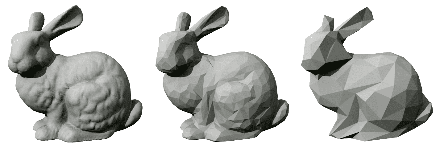
Mesh storage
In a triangle mesh, the vertices are stored in an ordered list
P_k, with k =
1\ldots N.
Triangles are represented by a triplet of integer indices i_1, i_2, i_3 which represents the position
of the vertices P_{i_1}, P_{i_2},
P_{i_3} in the ordered list.
If 32-bit integers are used to store the indices, each triangle
requires 3×4 = 12 bytes.
This approach is highly efficient, since vertices are typically
shared by multiple adjacent triangles. And it’s easier to move vertices
in 3D space!
Model: 44,000 vertices, 80,000 triangles.
(u, v) Coordinates
In the case of an arbitrary mesh, there are infinitely many
possible ways to create a (u, v)
mapping on the surface.
In meshes, each element of the mesh is made to cover a
specific portion of the entire space [0, 1]
\times [0, 1].
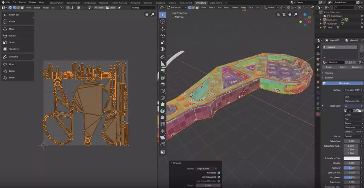
3D modeling programs like Blender allow you to modify the (u, v) mapping of each element.
Ray Intersection
Calculating the intersection between a mesh and a ray is not easy
to implement.
The bottleneck in solving the rendering equation is typically the
time spent on ray-shape intersections.
As the number of shapes increases, the computation time
necessarily increases as well as O(N).
An effective optimization is the use of bounding boxes, which
rely on the concept of “axis-aligned box”. Let’s start from the
latter.
Axis-aligned boxes
The cubic shape is not very interesting in itself, but it lends
itself to some optimizations relevant for polygonal meshes.
Due to its particular purpose, we will treat the case of cubes
using different conventions than those made for spheres and planes:
- We will not limit ourselves to the unit cube with a vertex at the
origin…
- …but we will assume that the faces are parallel to the coordinate
planes.
These assumptions are referred to in the literature as
axis-aligned bounding box (AABB).
In-memory representation
A box with edges aligned along the xyz axes can be defined by the following
quantities:
- The minimum and maximum x
values;
- The minimum and maximum y
values;
- The minimum and maximum z
values.
Equivalently, you can store two opposite vertices of the
parallelepiped, P_m (minimum values of
x, y
and z) and P_M (maximum values).
Ray-AABB intersection
Let’s write the ray as r: O + t \vec
d.
The calculation for the 3D case is very similar to the 2D case,
so let’s consider the latter:
![]()
Ray-AABB intersection
Let F_i be a generic point on a
face of the box perpendicular to the i-th direction (six planes in total), which
will have coordinates
F_0 = (f_0^{\text{min}/\text{max}}, \cdot, \cdot), \quad F_1 = (\cdot,
f_1^{\text{min}/\text{max}}, \cdot), \quad F_2 = (\cdot, \cdot,
f_2^{\text{min}/\text{max}}).
In general, there are two ray-face intersection along
the i-th coordinate, if we consider
whole planes instead of the actual faces:
O + t_i \vec d = F^{\text{min}/\text{max}}_i\quad\Rightarrow\quad
t_i^{\text{min}/\text{max}} = \frac{f_i^{\text{min}/\text{max}} -
O_i}{d_i}.
Ray-AABB intersection
Each direction produces two intersections, so in total there are
six potential intersections (one for each face of the cube).
But not all intersections are correct: they are calculated for
the entire infinite plane on which the face of the cube lies.
It is therefore necessary to verify for each value of t if the corresponding point P actually lies on one of the faces of the
cube.
Ray-AABB intersection
- In the case of the previous image, where the ray intersects the
parallelepiped, the intervals [t^{(1)}_i,
t^{(2)}_i] have a common section:
![]()
- The intersection of the intervals is an interval whose extremes
correspond to the intersection points of the ray with the AABB.
Ray-AABB intersection
- In the case where the ray misses the parallelepiped, the intervals
[t^{(1)}_i, t^{(2)}_i] are
disjoint:
![]()
- Therefore, if the intersection of the intervals for the three axes
gives the empty set, the ray does not hit the AABB.
Rendering complexity
Last week we implemented the World type, which
contains a list of objects
When calculating an intersection with an object,
World.ray_intersection must iterate over all the
Shapes in World
If you increase the number of Shapes tenfold, the
time required to produce an image also increases tenfold…
…but even solving the rendering equation in simple cases can take
hours!
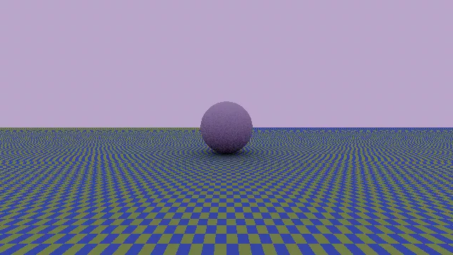
![]()
This image contains three geometric shapes (two planes and a sphere),
and was calculated in ~156 seconds by a code written in a compiled
language (FreePascal).
Optimizations
With our implementation of World, the time required
to compute an image is roughly proportional to the number of ray-shape
intersections.
But realistic scenes contain many shapes!
Moana island scene is a scene composed of ~15 billion
basic shapes. The rendering time would be on the order of 25,000
years!
Now that we have described axis-aligned boxes, let’s move to the
concept of axis-aligned bounding boxes, which provides a simple
but effective optimization.
Axis-aligned bounding box
Axis-aligned bounding boxes (AABBs) are AABBs that
delimit the volume occupied by objects.
They are widely used in computer graphics as an
optimization mechanism.
The principle is as follows:
- For each shape in space, its AABB is calculated;
- When determining the intersection between a ray and a shape, it is
first checked whether the ray intersects the AABB;
- If it does not intersect, we move on to the next shape, otherwise we
proceed with the intersection calculation.
![]()
Usefulness of AABBs
AABBs are useful only for scenes made up of many objects. For
simple scenes, they can introduce unnecessary overhead.
They are however very useful with triangle meshes and
complex CSG objects.
If you want to support AABBs in your ray-tracer, you should add
an aabb member to the Shape type to be used
inside Shape.rayIntersection:
class MyComplexShape:
    # ...
    def rayIntersection(self, ray: Ray) -> Optional[HitRecord]:
        inv_ray = ray.transform(self.transformation.inverse())
        if not self.aabb.quickRayIntersection(inv_ray):
            return None

        # etc.
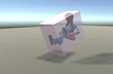
AABB and meshes
AABBs are perfect for applying to meshes. (In this case
they obviously do not apply to the individual elements,
but to the mesh as a whole).
When loading a mesh, its AABB can be calculated by calculating
the minimum and maximum values of the coordinates of all
vertices.
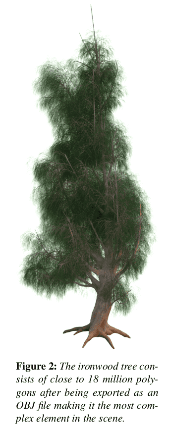
In the case of the Oceania tree, the intersection
between a ray and the 18 million elements would only occur for those
rays actually oriented towards that tree.
Beyond AABBs
However, it is not always sufficient to use AABBs for
meshes to be efficient.
Scenes are often almost completely occupied by a few complex
objects, and in this case AABBs do not provide any advantage (as in the
previous image).
However, there are several sophisticated optimizations that
transform the problem of looking for ray-triangle hits from O(N) to O(\log_2
N). The most common acceleration structures are KD-trees and Bounding
Volume Hierarchies (see this
video by Sebastian Lague). They are both explained in the book
by Pharr, Jakob & Humphreys.
Introduction to Debugging
Last week you fixed your first bug, which concerned the incorrect
orientation of the images saved by your code.
In general, a bug is a problem in the program that makes
it work differently than expected.
It is very important to have a scientific approach to bug
management! In the next slides I will give you some general
guidelines.
Fault, Infection, and Failure
Zeller’s excellent book Why Programs Fail: A Guide
to Systematic Debugging categorizes the manifestation of a
bug into three distinct stages:
- Fault: an error in the way the code is
written;
- Infection: a certain input “activates” the fault
and alters the value of some variables compared to the expected
case;
- Failure: the outcome of the program is wrong,
either because the results are incorrect, or because the program
crashes.
The bug lies in the initial fault, but if there is no
infection or no failure, it is difficult to notice it!
Example
In your second-year, you implemented code that calculates the
value of
\int_0^\pi \sin x\,\mathrm{d}x
using Simpson’s rule:
\int_a^b f(x)\,\mathrm{d}x \approx \frac{h}3 \left[f(a) +
4\sum_{i=1}^{n/2} f\bigl(x_{2i-1}\bigr) + 2\sum_{i=1}^{n/2 - 1}
f\bigl(x_{2i}\bigr) + f(b)\right].
Often the implementation is wrong even though the result is
correct (\int = 2)!
\int_a^b f(x)\,\mathrm{d}x \approx \frac{h}3 \left[f(a)+
{\color{red}{4}}\sum_{i=1}^{n/2} f\bigl(x_{2i-1}\bigr) +
{\color{red}{2}}\sum_{i=1}^{n/2 - 1} f\bigl(x_{2i}\bigr) + f(b)\right].
Often students swap the 4 with the 2.
This leads to an infection: the value of the expression
in square brackets is wrong.
This leads to a failure: the result of the integral is
wrong.
Of all the cases, this is the simplest: it is immediately obvious
what the problem is!
\int_a^b f(x)\,\mathrm{d}x \approx \frac{h}3 \left[f(a)+
4\sum_{i=1}^{\color{red}{n/2}} f\bigl(x_{2i-1}\bigr) +
2\sum_{i=1}^{\color{red}{n/2 - 1}} f\bigl(x_{2i}\bigr) + f(b)\right].
Sometimes students terminate one of the two summations too early
(they forget the last term) or too late (they add an extra
term).
In the case of \int_0^\pi \sin
x\,\mathrm{d}x, the last term of the summation is for x \approx \pi, so it is very small: there is
an infection, but if you print only a few significant digits on
the screen, the result may be rounded to the correct value, and
therefore there is no failure.
\int_a^b f(x)\,\mathrm{d}x \approx \frac{h}3 \left[{\color{red}{f(a)}}+
4\sum_{i=1}^{n/2} f\bigl(x_{2i-1}\bigr) + 2\sum_{i=1}^{n/2 - 1}
f\bigl(x_{2i}\bigr) + {\color{red}{f(b)}}\right].
Sometimes students forget to add f(a) and/or f(b), or they multiply them by 2 or
4.
However, in the case of \int_0^\pi \sin
x\,\mathrm{d}x, the value of the expression in square brackets is
still correct because f(0) = f(\pi) =
0.
In this case there is a fault but there is no
infection nor a failure: this is the most difficult
case to identify!
Duplicate Issues
It is very common for the same fault to lead to
different failures: this depends on the input data, the type of
action being performed with the program, etc.
It is therefore very common for users to open different
issues that are however caused by the same
fault.
Example: a crash in
Julia is caused by the combination of two previously reported
issues, which at first glance did not seem related.
GitHub allows you to assign the Duplicated label to
issues:

How to Report Issues
When you observe a failure and want to open an
issue, you must indicate:
- List of actions that led to the failure (including all inputs!)
- Program output
- Description of the expected behavior and the observed behavior
instead
This is because the developer must be able to
reproduce the failure in a controlled
environment to identify the fault that caused it.
If a user reports an issue to you without some of these things
being clear, do not hesitate to ask for more details.
GitHub allows you to configure an issue
template.
Identifying Faults Scientifically
- Observe/reproduce a failure
- Formulate a hypothesis about the fault that caused the
failure
- Use the hypothesis to predict where an infection might be visible
(e.g., using a debugger or
print statements). If the
observation contradicts the prediction, refine the hypothesis.
We have already seen this pattern many times with LLMs: you must
verify claims (ChatGPT’s output, reason for a fault) before
assuming they are true!
Using LLMs to debug codes
Today, LLMs can be very effective in finding some types of
errors
Example of a prompt:
The following C++ code should print all the numbers from 0 to 10 in steps of 2, so the expected output should be 0, 2, 4, 6, 8, 10. However the code fails to print 10:

    for (int i{}; i < 10; ++i) {
        println("{}", i);
    }

Can you help me in understanding why it does not work?
More advanced LLMs can acts as agents: they interact
with your build system to modify the code, compile it, run tests, and
iterate. Examples: Claude Code, Gemini
Code Assist…
Are they worth it?
Sometimes, they can be very useful!
However, they have the tendency to overdo changes
As described in the article Coding models are
doing too much, the authors purposefully injected some simple bugs
(e.g., changing < into <=) and then
asked the LLM to fix it. The result often overwrote the whole function
instead of just fixing that single character!
As I have said repeatedly, never trust a LLM
before having verified its suggestions!
Ethical considerations about bugs and bug reports
Claude Mythos Preview
Anthropic is a
key player in the LLM world. They produce very effective LLM agents like
Code, Sonnet, Opus, etc.
In April 2026, they announced their new product, Claude Mythos,
which seems to have incredible
potential:
- They discovered a 27-year-old (quite harmless) bug in OpenBSD, one of the most secure
Operating System on Earth;
- They discovered a 16-year-old bug in FFmpeg, which we learned to use just
a few days ago
This new tool has huge ethical implications (and raised
questions…), which Anthropic addressed by starting the Glasswing
project.
Project Glasswing
Instead of releasing Claude Mythos to the general public, they
decided to freely grant its usage (100 M$ tokens) to “selected partners”
like Microsoft, Apple, NVIDIA, The Linux Foundation, Broadcom,
etc.
Each partner will use Mythos to find and fix bugs in
their own codebase
The general public won’t have access to Claude Mythos: this
prevents malicious actors (hackers) from compromising critical
systems
How can hackers exploit a bug?
Consider this code:
float buffer[1024]; // This is large enough for any reasonable case
for(int i{}; i < nsamples; ++i) {
    buffer[i] = read_next_float();
}
The number 1024 was probably picked as a very large
limit, because in normal conditions the program will
never read more than this.
However, if you pass the wrong input and it’s too large, you will
overwrite the memory and likely cause a segmentation
fault
This turns out to be an annoyance, as the program crashes.
But…
How can hackers exploit a bug?
…what if the user is a malicious actor who wants
to take control of the machine?
A possible hacking technique here would be to pass 1024 floating
point numbers, followed by some specific machine code (the
payload)
The buffer variable resides on the stack, where
other crucial information about the program flow is saved (return
address of the function). By carefully injecting specific values after
the 1024 float-s, the hacker can overwrite the return
address and force the program to execute arbitrary code that can grant
the hacker access to the machine.
This bug is no longer an annoyance: it is a security
hole!
How does this affect you?
Even seemingly innocent bugs can have dangerous consequences and
open security holes.
LLMs did not create this problem, but by having the potential to
discover several of them all at once and with relatively little
effort, the problem is exhacerbated.
You might think this is relevant only for operating system
developers, but you are just targeting scientific software.
Do not be fooled! All of this can affect you as
well!
Let’s imagine a possible example
Suppose you developed a library to perform conversion between
coordinate systems (Cartesian, spherical, cylindrical, etc.)
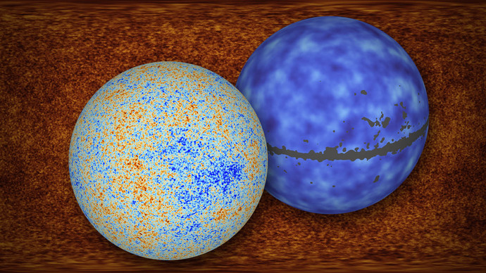
ESA wants to publish an interactive 3D viewer of Planck’s maps of
the Cosmic Microwave Background and internally uses your library in a
web app
![]()
However, your library has a zero-day
vulnerability, i.e., a bug that nobody discovered yet. This bug
works similarly to what we just described: it lets malicious actors run
arbitrary code on the machine hosting the web app.
The malicious actors execute a payload to gain a remote
shell
Being an ESA machine, the webserver is likely connected with the
internal network
ESA and EUMETSAT develop weather satellites like METEOSAT and
MetOp, and their data likely land on some of the computers in this
schema
Once a malicious actor has access to satellite data, several bad
things can happen:
Access to raw data before they are processed and filtered (e.g.,
to find minute erosion signs in dams or gas reservoirs)
Modification/removal of existing data (e.g., hiding hints that a
hurricane is forming near a densely inhabited area)
All of this because of a bug in a seemingly harmless numerical
library any of us could have developed!
Cyberwarfare
In modern times, a new idea of warfare emerged: the
“cyberwarfare”
One of the most studied cases in literature is Russia, as its
leaders have repeatedly talked about this concept (the so-called “Gerasimov
doctrine”)
With cyberwarfare, the boundary between “war” and “pace” becomes
less definite
It is well explained in the book Brigate
russe (Marta Ottaviani, ed. Bompiani)
Cyberwarfare
In cyberwarfare, you employ cyber capabilities to attack your
enemy:
- Spread of fake news through social media and mass media
- Espionage and sabotage of critical infrastructure
- → Cyberattacks ←
Historically, Russia was the first country to invest in this
because of the possibility to fill the huge gap with the raw military
power of other countries like China and the US (cyberwarfare is much
cheaper!)
How to prevent these attacks?
EU is allocating significant resources in cyberdefense:
- Cyber
Resilience Act (CRA): mandatory security requirements for digital
products sold in Europe (December 2024)
- Cyber
Solidarity Act (CSA): ~1 G€ to fund a system that uses AI to spot
cyberattacks as soon as possible (Cybersecurity Alert System),
implements a system that can substitute essential systems compromised by
an attack (Cybersecurity Emergency Mechanism), and establishes
a mechanism to review past incidents (Cybersecurity Incident Review
Mechanism)
Apart from these institutional measures, what can one do to
improve cybersecurity?
Bug reporting
The potential impact of bugs in one’s own code cannot be
determined easily
It is extremely important to fix bugs in your code…
…but, as we just saw, it is equally important to report
bugs to others as well!
Open-source projects usually encourage people to provide pull
requests to fix issues. But what about closed-source programs like
Microsoft Windows, Adobe Photoshop, Google Sheet…?
Report bugs in commercial software
Hopefully, these failures in handling bug reports are becoming
rarer and rarer
In general, do not report the bug on social media or
your website! Think that you are protecting users, not only the firm.
Instead, inform the firm through private channels (big firms usually
have a “Vulnerability Disclosure Policy”, which offer legal protections
for contributors)
You should give them some time to acknowledge the bug and fix it.
After a grace period (usually 90 days), you can probably disclose the
bug
Some firms organize bug bounty
programs