Geometric Shapes

«Cornell box»

Rendering Equation

• To solve the rendering equation, we need to trace the path of light rays in three-dimensional space and solve the rendering equation:

  \begin{aligned} L(x \rightarrow \Theta) = &L_e(x \rightarrow \Theta) +\\ &\int_{4\pi} f_r(x, \Psi \rightarrow \Theta)\,L(x \leftarrow \Psi)\,\cos(N_x, \Psi)\,\mathrm{d}\omega_\Psi, \end{aligned}

• The integral is calculated over the solid angle, and it is not very convenient for the numerical solution of the problem: we will have a list of objects, not solid angles, to iterate over.

• Therefore, we look for an alternative formulation that makes things simpler.

Alternative Form

• Let’s focus on the most complex term of the equation, i.e., the integral:

  \int_{4\pi} f_r(x, \Psi \rightarrow \Theta)\,L(x \leftarrow \Psi)\,\cos(N_x, \Psi)\,\mathrm{d}\omega_\Psi.

• The integral is calculated over the entire solid angle 4π, and its physical meaning is to take into account the radiation falling on point x of a surface.

• This radiation must have been emitted by some surface element \mathrm{d}\sigma' on the scene, corresponding to a point x' in space (see the following figure).

Alternative Form

• By definition of solid angle, therefore, \mathrm{d}\omega_\Psi is written as follows:

  \mathrm{d}\omega_\Psi = \frac{\mathrm{d}\sigma'\,\cos\theta_i'}{\left\|x - x'\right\|^2}.

• The integral term of the rendering equation can therefore be rewritten as follows:

  \int_{\sum S} f_r(x, \Psi \rightarrow \Theta)\,L(x, x - x')\,\frac{\cos\theta_i\,\cos\theta'}{\left\|x - x'\right\|^2}\mathrm{d}\sigma',

  where \sum S indicates all surfaces visible from x.

Visibility Function

• To resolve this ambiguity, a visibility function v(x, x') is usually introduced, defined as follows:

  v(x, x') = \begin{cases} 1\ &\text{ if $x'$ is visible from $x$,}\\ 0\ &\text{ if $x'$ is not visible from $x$.} \end{cases}

• In this way, the integral is rewritten over the entire set of points x':

  \int_{\forall x' \in \sum S} f_r(x, \Psi \rightarrow \Theta)\,L(x, x - x')\,\frac{\cos\theta_i\,\cos\theta'}{\left\|x - x'\right\|^2}\,v(x, x')\,\mathrm{d}\sigma'.

Rays and Geometric Shapes

• We see that in a ray-tracing code it is necessary to be able to perform these calculations:

  1. Intersection between a ray and a surface;
  2. Determination of the visibility function v(x, x') between two points.

• These two problems can be solved in a very similar way, and that is what we will see in today’s lesson.

Ray/Shape Intersections

Representation of Shapes

• In a ray-tracer, surfaces are represented by analytical equations.

• The intersection between light rays and shapes is calculated using the rules of analytic geometry:

  1. Rays and shapes are represented as equations where the unknown is the point (x, y, z) in space.
  2. The system of equations for the ray and for the shape is solved, in order to find the points (x, y, z) in common between the two equations.

• Thanks to our implementation of affine transformations, we can implement only the simplest shapes, which can then be modified through concatenations of transformations.

Transformations

• Usually geometric shapes are expressed in complex forms; for example, the unit sphere is represented by an implicit equation:

  x^2 + y^2 + z^2 = 1.

• However, we know how to apply a transformation T only to points, vectors, and normals, not to implicit equations.

• It is more convenient to apply the inverse transformation to the light rays: if T transforms the “privileged” reference frame of a shape into the real world system, T^{-1} can transform a ray O + t \vec d in the real world system into the privileged one of the shape.

Transforming Rays

• Suppose that T is the transformation to be applied to the surface S. The transformed surface T\cdot S is then the set of points

  T\cdot S = \left\{T x: x \in S\right\},

• If the ray O + t \vec d intersects T\cdot S when t = \tilde t, then

  O + \tilde t \vec d = T \tilde x,\ \Rightarrow\ T^{-1} O + \tilde t\,T^{-1} \vec d = \tilde x,

  which is equivalent to formulating the intersection problem in the reference frame of S. Note that \tilde t does not change between the two formulations!

Types of Shapes

• In this course we will discuss the following geometric shapes:

  1. Spheres;
  2. Planes;
  3. Constructive Solid Geometry (CSG);
  4. Triangles;
  5. Meshes.

• We will deal with triangle meshes and cubes next week, since they are usually associated with more advanced topics (bounding boxes and triangle meshes).

Spheres

Unit Sphere

• The equation of a three-dimensional sphere with center C and radius R is

  (x - c_x)^2 + (y - c_y)^2 + (z - c_z)^2 = R^2,

  and it derives from the geometric definition of a sphere.

• But we will just consider the unit sphere centered at the origin:

  x^2 + y^2 + z^2 = 1\ \rightarrow\ \left\|P - 0\right\|^2 = (P - 0) \cdot (P - 0) = 1,

  where 0 is the origin of the axes and P is a generic point on the sphere. We can then translate and transform it into an ellipsoid using a transformation T.

Ray-Sphere Intersection

• Determining the intersection between a ray and a sphere requires solving the following equations simultaneously:

  \begin{cases} (P - 0) \cdot (P - 0) = 1,\\ P = O + t \vec d, \end{cases}

• The unknowns are P and t; the latter is the distance from the origin of the ray at which the intersection with the sphere occurs.

Solving the Equation

• We can find t by substituting the second equation into the first:

  (O + t\vec d - 0) \cdot (O + t\vec d - 0) - 1 = 0.

• The notation O - 0 simply indicates that O should be considered a vector rather than a point. We simplify the notation as follows:

  O - 0 = \vec O,

  which suggests that we can use the Point.toVec() function/method.

Solving the Equation

• Expanding the definition of the dot product, we obtain

  t^2 \left\|\vec d\right\|^2 + 2 t\,\vec O \cdot \vec d + \left\|\vec O\right\|^2 - 1 = 0,

• This is a quadratic equation, and therefore admits zero, one, or two solutions:

  1. Zero solutions: the ray does not intersect the sphere;
  2. One solution: the ray is tangent to the sphere;
  3. Two solutions: the ray intersects the sphere, passes through it, and intersects its surface on the opposite side.

Ray-Sphere Intersections

• To distinguish between the three cases, we need the discriminant:

  \frac\Delta4 = \left(\vec O \cdot \vec d\right)^2 - \left\|\vec d\right\|^2\cdot \left(\left\|\vec O\right\|^2 - 1\right).

• In the case where \Delta > 0, the two intersections are

  t = \begin{cases} t_1 &= \frac{-\vec O \cdot d - \sqrt{\Delta / 4}}{\left\|\vec d\right\|^2},\\ t_2 &= \frac{-\vec O \cdot d + \sqrt{\Delta / 4}}{\left\|\vec d\right\|^2}. \end{cases}

Invalid Intersections

• Not all intersections between a ray and a sphere are valid: it also depends on the starting point of the ray.

• Furthermore, it doesn’t make much sense to consider tangent intersections, so we will ignore them.

Valid Intersections

• The criterion for deciding whether an intersection is valid also depends on the values t_\text{min} and t_\text{max} of the ray O + t \vec d.

• Putting together everything we have said so far, an intersection for t = \tilde t is valid if and only if

  t_\text{min} \leq \tilde t \leq t_\text{max}

  (using < instead of ≤ doesn’t change anything).

• If both intersections t_1 and t_2 satisfy this criterion, then the smaller of the two is considered, i.e., t_1 (visibility criterion).

Beyond Intersections

• Once t and consequently the point P have been identified, the work is not yet finished.

• To apply the BRDF f_r to the point, it is also necessary to know the normal \hat n to the surface.

• Furthermore, in general, the BRDF of a surface depends on the exact point of intersection, which for a surface is usually indicated as a two-dimensional point (u, v).

• Let’s look at these two aspects in detail, starting with the normal.

Normal of a Sphere

• Given a point P, any radius is always normal to the surface of the sphere, so it is easy to determine the normal at point P:

  \hat n_P = P - C,

  where C is the center of the sphere.

• However, there is an ambiguity in the sign: both P - C and C - P are normal to the surface. But should the normal be inward or outward?

Normal of a Sphere

• The choice of the normal depends on the direction of arrival \vec d of the ray.

• We can therefore check the sign of

  \hat n \cdot \vec d = \left\|\hat n\right\|\cdot\left\|\vec d\right\|\,\cos\theta,

  and if it is positive, we consider -\hat n instead of \hat n.

Intersection Point

• Once the intersection point P between the sphere and the ray is determined, it is usually necessary to estimate the BRDF at P.

• But it is inconvenient to do so if P is expressed in 3D coordinates!

Intersection Point

• Rather than the point P, it is necessary to know the position in two-dimensional coordinates on the surface of the sphere.

• In the specific case of the sphere, we can use the latitude-longitude pair

• In the general case of a surface S, we will always seek for two-dimensional parameterizations (u, v).

Surface of the Sphere

• Given a point P on the surface of the sphere, we can derive the colatitude \theta and the longitude \phi using trigonometry:

  \theta = \arccos p_z, \quad \phi = \arctan \frac{p_y}{p_x}.

• The range of values \theta \in [0, \pi], \phi \in [0, 2\pi] is too specific for the sphere, so we can use this parameterization:

  u = \frac\phi{2\pi} = \frac{\arctan p_y / p_x}{2\pi}, \quad v = \frac\theta\pi = \frac{\arccos p_z}\pi.

Planes

Infinite Plane

• In affine geometry, a plane is defined by its normal vector \hat n and a point O through which the plane passes:

  (P - O) \cdot \hat n = 0,

  where P is a generic point on the plane.

• (As you can guess, in algebraic geometry, planes are represented by bivectors: calculations are much simpler, especially if you employ projective geometric algebra!)

Standard Plane

• Since we can exploit transformations, we study the particular plane that passes through the origin and is generated by the x and y axes (i.e., it is perpendicular to the z axis).

• In this case

  (P - O) \cdot \hat n = 0\ \Rightarrow\ \vec P \cdot \hat e_z = 0,

  which is equivalent to requiring that

  P_z = 0.

Ray-Plane Intersection

• The intersection between the plane and the ray O + t \vec d is therefore trivially simple: just require that the z component of the point along the ray vanishes for some value of t.

• The analytical solution is

  O_z + t d_z = 0\ \Rightarrow\ t = -\frac{O_z}{d_z},

  which is obviously valid only if d_z \not= 0, i.e., if the direction \vec d of the ray is not parallel to the xy plane.

Normals

• The normal of the plane is obviously \pm \hat e_z, where the sign is determined by the same rule used for the sphere.

• But in the case of the plane, the formula is even simpler: if \vec d is the direction of the ray, then the condition for changing the sign becomes

  \vec d \cdot \hat n < 0\ \Rightarrow\ d_z < 0.

Parameterization of the Plane

• Unlike the sphere, a plane is an infinite surface.

• In this case, the plane is parameterized with periodic conditions:

  u = p_x - \lfloor p_x \rfloor,\quad v = p_y - \lfloor p_y \rfloor,

  where \lfloor \cdot \rfloor indicates the floor function, so that u, v \in [0, 1) as in the case of the sphere.

• The entire surface of the plane is therefore the periodic repetition of the region [0, 1] \times [0, 1] (tile pattern).

Parameterization of the plane

Constructive Solid Geometry

Constructive Solid Geometry

• The shapes seen so far are very simple: spheres and planes.

• We will see in the future that arbitrarily complex shapes can be approximated with sets of triangles, but handling this kind of shape efficiently is complex!

• Today we present a simple technique to construct complex geometric shapes starting from simple shapes: Constructive Solid Geometry (CSG).

Set Operations

• Union
• Difference
• Intersection

Union

• The intersections with all the shapes are determined;
• The closest intersection is chosen, assigning it the BRDF of the corresponding shape.

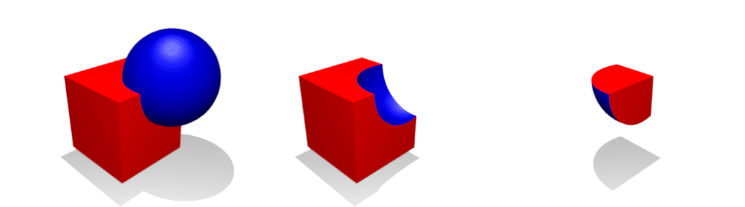
Difference

• The intersections with the shapes are determined;
• The intersections internal to shape #2 (C) and those on the surface of #2 that are not internal to #1 (D) are omitted.

Intersection

• The intersections with the shapes are determined;
• Only the intersections in one of the two shapes that are internal to the other shape are considered (point B intersects #2 and is internal to #1, C intersects #1 and is internal to #2).

Fusion

• It works like a union, but the internal points B and C are not considered.
• It is only useful for semi-transparent materials.

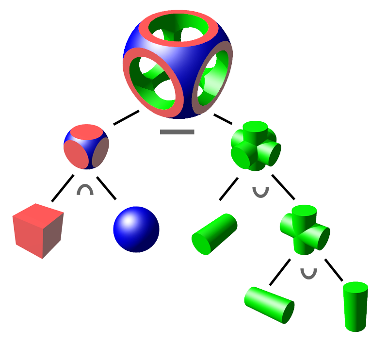
Hierarchies

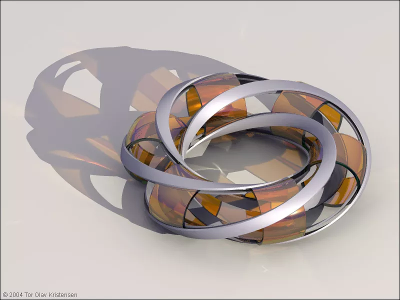
Villarceau Circles, by Tor Olav Kristensen (2004)

Triangles and quadrilaterals

3D Modeling

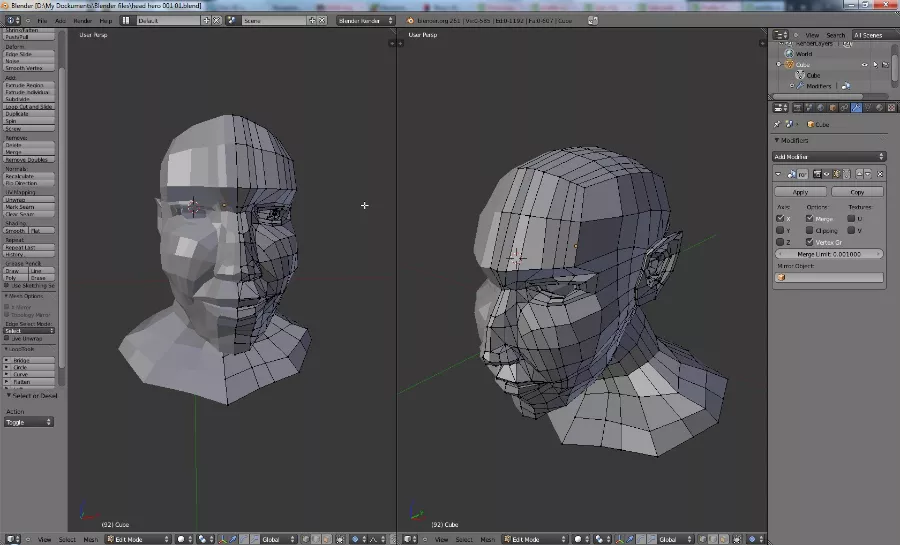
3D Scanners

Stanford bunny (1994)

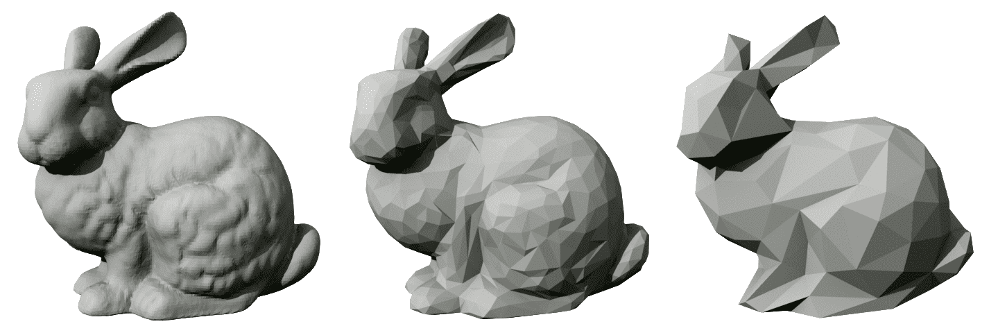
(Model obtained from the scan of a ceramic statuette)

Triangles

Triangles are a geometric shape widely used in 3D modeling and rendering programs, due to their many properties:

1. They are the planar surface with the fewest vertices (→ efficient to store).
2. Their representation in space is unique (one and only one planar triangle passes through three points).
3. Their surface is parameterizable in (u, v) coordinates in a very simple way.
4. Complex surfaces can be represented as a union of multiple triangles.

Barycentric Coordinates

• Barycentric coordinates were proposed by Möbius in 1827. They express the points of a plane passing through the points A, B, C by means of the expression

  P(\alpha, \beta, \gamma) = \alpha A + \beta B + \gamma C,

  where \alpha, \beta, \gamma \in \mathbb{R} are the barycentric coordinates.

• Barycentric coordinates are very useful for characterizing the triangle with vertices A, B, C: the point P is inside the triangle if and only if

  0 \le \alpha \le 1,\quad 0 \le \beta \le 1,\quad 0 \le \gamma \le 1, \quad \alpha + \beta + \gamma = 1.

Coordinates in Triangles

• The condition \alpha + \beta + \gamma = 1 means that the points of a triangle are characterized by two degrees of freedom, as it should be for a two-dimensional surface.

• Equality in the first three inequalities holds for the points along the edge of the triangle.

• Using the last equality, a more meaningful form is obtained:

  P(\beta, \gamma) = A + \beta(B - A) + \gamma(C - A) = A + \beta \vec v_{AB} + \gamma \vec v_{AC},

  which expresses P as A plus a displacement towards B and one towards C.

Coordinates in Triangles

• It can be shown that the barycentric coordinates of a point P are related to the area \sigma of the triangle and to the areas of the three sub-triangles having as vertex the point P and two of the vertices:

  \alpha = \frac{\sigma_1}\sigma = 1 - \frac{\sigma_2 + \sigma_3}\sigma, \quad \beta = \frac{\sigma_2}\sigma, \quad \gamma = \frac{\sigma_3}\sigma.

• If a negative sign is assigned to the areas that are outside the triangle, these equations hold for any point on the plane in which the triangle lies.

Interactive Example

Quadrilaterals

• We will focus on triangles today, but rendering programs also offer the possibility of defining quadrilaterals.

• If we limit ourselves to parallelograms, they can be represented as the union of a vertex P and two vectors \vec v and \vec w; in this way, the results that we will show today are easily extendable to them as well:

Ray Intersection

• Let’s now see how to use barycentric coordinates to efficiently calculate the intersection between a triangle and a ray.

• Unlike what we did with spheres and planes, in this case we will not adopt a simplified reference system. The reason will be clear when we explain triangle meshes.

• We will therefore identify a triangle by the coordinates of the three points A, B, C (nine floating-point values).

The Analytical Problem

• Consider the ray r(t): O + t \vec d and the generic point P(\beta, \gamma) of the triangle. The intersection is given by

  A + \beta (B - A) + \gamma (C - A) = O + t \vec d,

  with the constraint 0 \leq (\beta, \gamma) \leq 1.

• Let’s rearrange the equation to move the three unknowns \beta, \gamma and t to the left:

  \beta (B - A) + \gamma (C - A) - t \vec d = O - A.

Matrix Form

• The equation we obtained is

  \beta (B - A) + \gamma (C - A) - t \vec d = O - A,

  which is a vector equation in the three components x, y, z.

• In matrix form, the system can be rewritten as follows:

  \begin{pmatrix} b_x - a_x& c_x - a_x& -d_x\\ b_y - a_y& c_y - a_y& -d_y\\ b_z - a_z& c_z - a_z& -d_z\\ \end{pmatrix} \begin{pmatrix} \beta\\\gamma\\t \end{pmatrix} = \begin{pmatrix} o_x - a_x\\o_y - a_y\\o_z - a_z \end{pmatrix}.

Analytical Solution

• The solution depends on the determinant of the matrix M:

  \det M = \det \begin{pmatrix} b_x - a_x& c_x - a_x& d_x\\ b_y - a_y& c_y - a_y& d_y\\ b_z - a_z& c_z - a_z& d_z\\ \end{pmatrix},

  which must be different from zero, otherwise the ray is parallel to the plane of the triangle.

• The solution is easily obtained with Cramer’s rule, which is inefficient in the general case but adequate for 3×3 matrices as the one above.

Analytical Solution

• Obviously, once the solution is obtained it is necessary to verify that

  t_\text{min} < t < t_\text{max}, \quad 0 \leq \beta \leq 1, \quad 0 \leq \gamma \leq 1.

• The normal of the triangle can be easily obtained from the cross product between the two vectors aligned with the sides:

  \hat n = \pm (B - A) \times (C - A),

  where the sign is determined by the direction of the ray.

• The (u, v) coordinates can be set equal to (\beta, \gamma).