Animations

Creating animations

• The mathematics of transformations that we introduced in the last lesson allows us to easily create static images.

• What would change if we wanted to create animations instead? (We limit to the case where we only animate transformations.)

• Let’s see a practical example.

Transformations over time (1/2)

• Consider a 3D object centered at the origin.

• Imagine that at time t = 0 of the animation the object must be at position \vec k_0, and at time t = 1 at position \vec k_1.

• If I want to generate the frame of the object at a generic time 0 \leq t \leq 1, the transformation A is trivially

  A(t) = T_{\vec k_0 + (\vec k_1 - \vec k_0) t} = \begin{pmatrix} 1&0&0&k_{0x} + (k_{1x} - k_{0x})t\\ 0&1&0&k_{0y} + (k_{1y} - k_{0y})t\\ 0&0&1&k_{0z} + (k_{1z} - k_{0z})t\\ 0&0&0&1 \end{pmatrix}.

Transformations over time (2/2)

• Scaling transformation are equally trivial to animate: to scale from s_0 to s_1, I can define \xi(t) = s_0 + (s_1 - s_0) t

• The transformation is

  A(t) = M_{s_0 + (s_1 - s_0) t} = M_{\xi(t)} = \begin{pmatrix} \xi(t)&0&0&0\\ 0&\xi(t)&0&0\\ 0&0&\xi(t)&0\\ 0&0&0&1 \end{pmatrix}.

Animating rotations

• Rotations are represented through orthogonal matrices (R(t) R(t)^t = I).

• We cannot interpolate the coefficients of two rotation matrices with two arbitrary axes \vec a_1 and \vec a_2 R(0) = \begin{pmatrix} m_{11}&m_{12}&m_{13}\\ m_{21}&m_{22}&m_{23}\\ m_{31}&m_{32}&m_{33} \end{pmatrix},\ % R(1) = \begin{pmatrix} m'_{11}&m'_{12}&m'_{13}\\ m'_{21}&m'_{22}&m'_{23}\\ m'_{31}&m'_{32}&m'_{33} \end{pmatrix},\quad with the usual formula m_{ij} + \bigl(m'_{ij} - m_{ij}\bigr) t: the resulting R(t) is not orthogonal!

Example

Example

• The Planck satellite had a star tracker on board that identified the satellite’s orientation with respect to the fixed stars.

• The orientation (attitude) was measured 10 times per second (the scientific data were sampled ~100 times per second) and transmitted to the ground station:

• On the ground, the orientation is needed at the same sampling rate as the scientific data, so interpolation is necessary.

• To do this, the Planck data reduction pipeline used quaternions.

Complex Numbers and Quaternions

Complex Numbers and Quaternions

• We already expressed rotations in matrix form.

• It is also possible to express rotations using complex numbers (in 2D) or quaternions (in 3D).

• Quaternions have many advantages over 3D rotation matrices and are used in many fields.

• If you want to learn more, two excellent texts are Visualizing quaternions (A. J. Hanson) and Quaternions for computer graphics (J. A. Vince).

Complex Numbers

• The algebra ℂ of complex numbers contains elements z = (\Re z, \Im z) = (x, y).

• The product is defined as

  z_1 \cdot z_2 = (\Re z_1\,\Re z_2 - \Im z_1\,\Im z_2, \Re z_1\,\Im z_2 + \Im z_1\,\Re z_2).

• Introducing i such that i^2 = -1 and writing complex numbers in the form z = x + i y, the product formula is easier to remember:

  (x_1 + i y_1) \cdot (x_2 + i y_2) = x_1 x_2 - y_1 y_2 + i \bigl(x_1 y_2 + x_2 y_1\bigr).

Rotations and Complex Numbers

• On the plane, it is possible to encode a rotation R(\theta) around the origin using the complex number

  r(\theta) = e^{i \theta} = \cos\theta + i\sin\theta

  if the vector \vec{v} = x \hat e_x + y \hat e_y to be rotated is associated with the complex number

  z = x + iy.

  Under these assumptions, the expression r(\theta) \cdot z is equivalent to R(\theta)\vec{v}.

• Instead of the 4 coefficients of the matrix R(\theta), only \Re z and \Im z are needed.

From 2D to 3D

• Quaternions generalize the ability of complex numbers to encode rotations in 3D. They were proposed by W. R. Hamilton (the one from the Hamiltonian) in 1843 precisely to extend ℂ (“invented” a few decades earlier), and their algebra is indicated by ℍ.

• If a complex number z is formed by two coefficients (the real part \Re z and the imaginary part \Im z), a quaternion q \in \mathbb{H} is composed of four coefficients:

  q = (q_0, q_1, q_2, q_3) = \bigl(q_0, \vec{q}\bigr),

  The term q_0 is called the scalar part, while \vec{q} = (q_1\ q_2\ q_3) is the vector part.

Quaternion Product

• The product p q between two quaternions is defined as follows:

  p q = \begin{pmatrix} p_0 q_0 - p_1 q_1 - p_2 q_2 - p_3 q_3\\ p_1 q_0 + p_0 q_1 + p_2 q_3 - p_3 q_2\\ p_2 q_0 + p_0 q_2 + p_3 q_1 - p_1 q_3\\ p_3 q_0 + p_0 q_3 + p_1 q_2 - p_2 q_1 \end{pmatrix}.

• This product satisfies all the properties of an associative algebra but is not commutative: p q \not= q p. (First algebra of this kind in history!).

• It is easy (but boring) to prove that \forall q\not=0 \in \mathbb{C} there is one and only one q^{-1} such that qq^{-1} = 1.

Notation for Quaternions

• Hamilton invented a very convenient notation for quaternions: q = q_0 + q_1 \mathbf{i} + q_2 \mathbf{j} + q_3 \mathbf{k}.

• If the following rules are defined, the product between quaternions from the previous slide follows consequently:

  \begin{aligned} \mathbf{i} \mathbf{i} &= -1, &\mathbf{i} \mathbf{j} &= \mathbf{k}, &\quad\mathbf{j} \mathbf{i} = -\mathbf{k},\\ \mathbf{j} \mathbf{j} &= -1, &\mathbf{j} \mathbf{k} &= \mathbf{i}, &\quad\mathbf{k} \mathbf{j} = -\mathbf{i},\\ \mathbf{k} \mathbf{k} &= -1, &\mathbf{k} \mathbf{i} &= \mathbf{j}, &\quad\mathbf{i} \mathbf{k} = -\mathbf{j}. \end{aligned}

Inner Product

• Like for complex numbers, quaternions have conjugates:

  q^* = (q_0, -q_1, -q_2, -q_3) = (q_0, -\vec{q}).

• It is possible to define an inner product between quaternions:

  p \cdot q = p_0 q_0 + p_1 q_1 + p_2 q_2 + p_3 q_3 = p_0 q_0 + \vec{p} \cdot \vec{q}.

• We can define a norm either through the inner product or through the conjugate:

  \left\|q\right\|^2 = q \cdot q = qq^* = q_0^2 + q_1^2 + q_2^2 + q_3^2 = q_0^2 + \left\|\vec{q}\right\|^2.

3D Rotations with Quaternions

• Given a normalized vector \hat n and an angle \theta, we associate with it the quaternion

  r(\theta, \hat n) = \left(\cos\frac\theta2, \sin\frac\theta2\,\hat n\right),

  which represents the rotation by an angle \theta around \hat n.

• Note that it looks similar to the complex rotor e^{i\theta} = \cos\theta + i\sin\theta, but with \theta/2 instead of \theta.

• If \left\|\hat n\right\| = 1, it obviously holds that \left\|r(\theta, \hat n)\right\| = 1.

Applying the Rotation

• A generic vector \vec v is rotated into \vec v' through this product of three quaternions:

  \vec v' = r(\theta, \hat n) \cdot (0, \vec v) \cdot r^{-1}(\theta, \hat n), where (0, \vec v) represents the quaternion associated with \vec v.

• Intuitively, r(\theta, \hat n) appears twice in the formula because it depends on the angle \theta/2, and not simply on the angle \theta.

• From the formula, it is evident that r(\theta, \hat n) and -r(\theta, \hat n) represent the “same” rotation (90 clockwise vs. 270° counterclockwise).

Are Quaternions Efficient?

• A rotation matrix must be stored by saving 9 coefficients in memory, while a quaternion requires only 4.

• Should we therefore use quaternions to represent rotations in our code?

• Generally no! If you explicitly write the sequence of operations needed to rotate a vector, you’ll see that the matrix representation requires fewer calculations.

• What are quaternions useful for, then?

Slerp

• The term slerp refers to the interpolation r(t) between two rotations r_1 and r_2.

• The formula for r(t) \in \mathbb{H} for t \in [0, 1] is simply

  r(t) = \frac{\sin\bigl((1 - t)\theta\bigr)}{\sin\theta}r_1 + \frac{\sin (t\theta)}{\sin\theta}r_2,

  where \theta is the “angle” between r_1 and r_2 (with \left\|r_1\right\| = \left\|r_2\right\| = 1):

  \theta = \arccos r_1 \cdot r_2.

• It is easy to show that r(t) represents a rotation \forall t\in [0, 1].

Example of Slerp

Animating Transformations

• Representing rotations with quaternions fills the last missing “hole”: all the transformations presented in the previous lesson are easily interpolable:

  1. Translations;
  2. Scale transformations;
  3. Rotations 🥳.

• The page Look, Ma, No Matrices! shows a nice example…

• …which uses an extension of the concept of “quaternion”, multivectors, to generate the effects shown at the bottom of the page.

• Let’s see then what multivectors and Clifford algebras are.

Clifford’s Algebras

Limits of Classical Geometry

• Vectors and pseudovectors follow different transformation rules.

• To describe rotations on a 2D plane, it is necessary to use 3D (pseudo)vectors, like angular momentum \vec{L} = \vec{r} \times \vec{p} or torque \vec{\tau} = \vec r \times \vec F.

• The cross product only exists in \mathbb{R}^3 (and \mathbb{R}^7, due to octonions…).

• The representation of rotations requires increasingly complicated algebras as the dimensions increase (complex numbers, quaternions…).

• It is not possible to invert products between vectors: if \vec a \times \vec x = \vec b with \vec a and \vec b known and x an unknown vector, there is no way to uniquely reconstruct \vec x.

Geometric Algebra

• Clifford algebras, and in particular geometric algebra, overcome all the problems listed in the previous slide.

• It is a branch of mathematics that rebuilds classical linear algebra and provides a more intuitive and coherent interpretation of certain geometric properties. Clifford proposed it in 1878.

• Geometric algebra is the application of Clifford algebras to the case of \mathbb{R}^n, and is what usually interests physicists. We will limit ourselves to these.

The Outer Product (or Grassman’s)

Product between Vectors

• The problem with the cross product \times is that it is defined only on ℝ³, while we desire a general algebra!

• In 1840, Hermann Günter Grassmann (1809–1877) defined the outer product \vec v \wedge \vec w between two vectors v and w (today also called the Grassmann product) as the oriented area on the plane \mathrm{Span}(\vec v, \vec w) with surface area

  \left\|\vec v\right\|\,\left\|\vec w\right\|\,\sin\theta.

Oriented Areas

• An oriented area like \vec v \wedge \vec w is called a bivector.

• Bivectors are oriented just like ordinary vectors: changing the sign of a bivector means reversing its direction of travel (∧ is antisymmetric).

• This is analogous to what happens with a vector: \vec v \rightarrow - \vec v.

• Just as a vector \vec v does not depend on the point of application, a bivector does not depend on its perimeter («shape»).

«Shape» of the Outer Product

It may sound strange! However, this guarantees that (2\vec v) \wedge \vec w = \vec v \wedge (2\vec w).

Meaning of the Outer Product

• This is the information encoded by an outer product \vec v \wedge \vec w:

  1. Extent of the surface (e.g., 15 m²);
  2. Inclination of the plane on which the surface lies;
  3. Orientation of the surface.

• This information is not encoded:

  1. Shape of the surface;
  2. Position of the plane with respect to the origin of the axes.

• It is possible to define scalar-bivector product and addition operations on bivectors: this makes them a vector space.

Scalar-Bivector Product

• The expression \lambda \vec v \wedge \vec w with \lambda \in \mathbb{R} is still a bivector.

• The area of \lambda \vec v \wedge \vec w is \left|\lambda\right| times the area of \vec v \wedge \vec w.

• If \lambda < 0, the direction is reversed, otherwise it remains the same.

Sum of Bivectors

Basis of Bivectors

• The sum appears geometrically complicated, but it enables the construction of a vector space.

• Being a vector space, it is possible to decompose bivectors using bases, and in this way the sum is trivial to understand: as simple as adding \vec v = 3\hat e_1 + 2\hat e_2 to \vec w = -2\hat e_1 + \hat e_2.

• We can define the canonical basis as the set of the three bivectors of unit area on the xy, yz and xz planes:

  \hat e_1 \wedge \hat e_2, \quad \hat e_2 \wedge \hat e_3, \quad \hat e_3 \wedge \hat e_1.

Basis of Bivectors

Sum of Bivectors

• Once we define a basis, the sum can be trivially defined in terms of the usual vector sum: if we have two bivectors

  \begin{aligned} \vec v &= 3 \hat e_1 \wedge \hat e_2 - \hat e_3 \wedge \hat e_1,\\ \vec w &= 2 \hat e_1 \wedge \hat e_2 + 4\hat e_3 \wedge \hat e_1,\\ \end{aligned}

  then their sum is

  \vec v + \vec w = 5\hat e_1 \wedge \hat e_2 + 3\hat e_3 \wedge \hat e_1.

• It is therefore trivial to perform calculations with bivectors!

Vector Product

• The outer product \vec u \wedge \vec v has some similarities with the classical cross product \vec u\times \vec v (we use the shorthand \hat e_j \wedge \hat e_k = \hat e_{jk}): \begin{aligned} \vec u \wedge \vec v &= (u_2 v_3 - u_3 v_2) \hat e_{23} + (u_3 v_1 - u_1 v_3) \hat e_{31} + (u_1 v_2 - u_2 v_1) \hat e_{12},\\ \vec u \times \vec v &= (u_2 v_3 - u_3 v_2) \hat e_1 + (u_3 v_1 - u_1 v_3) \hat e_2 + (u_1 v_2 - u_2 v_1) \hat e_3. \end{aligned}

• However, they are not the same: the outer product returns an oriented area, while the cross product returns an axial vector.

Outer and Vector Product

• It turns out that the physical laws that employ the × product can be interpreted more easily if we reformulate them as laws combining oriented areas.

• Moreover, the outer product has a number of advantages over the vector product:

  1. It is defined on \mathbb{R}^n for any n, while \times is only defined for n = 3.
  2. The outer product is associative, while the vector product is not: u \times (v \times w) \not= (u \times v) \times w. Calculations are therefore simpler.

Rotational Dynamics

• The angular momentum can be defined as the bivector \vec L = \vec r \wedge \vec p:

• Unlike the traditional definition (\vec L = \vec r \times \vec p), here \vec L represents an oriented section of a plane, which is intuitive: it is the plane on which the rotation takes place, and the orientation corresponds to the direction.

Reflections and Angular Momentum

• Remember the image that illustrated the reflection of pseudovectors?

• If L is a bivector, there is no problem! The plane on which the wheel rotates is perpendicular to the screen, and it is trivially reflected in the mirror.

Maxwell’s Equations

• How can we fix the weirdness in the following plot?

• Easy! We assume that \vec B is a bivector! (But \vec E is still a vector.)

Multivectors

Multivectors

• The outer product can also be calculated between a bivector and a vector, and we can exploit the associative property:

  \vec u \wedge \vec v \wedge \vec w = (\vec u \wedge \vec v) \wedge \vec w = \vec u \wedge (\vec v \wedge \vec w)

• The trivector \vec u \wedge \vec v \wedge \vec w represents an oriented volume.

• By repeatedly applying the outer product, we can generate trivectors, quadrivectors, etc. (This is why it is called outer).

• In general, we speak of multivectors, or k-vectors: a scalar is a 0-vector, vectors are 1-vectors, bivectors are 2-vectors, etc.

Examples

• Consider for example multivectors in ℝ³ using the canonical basis \left\{\hat e_i\right\}, and the usual shortcut \hat e_{ij\ldots} = \hat e_i \wedge \hat e_j \wedge \ldots:

  \begin{aligned} \hat e_{132} &= \hat e_1 \wedge (\hat e_3 \wedge \hat e_2) = -\hat e_1 \wedge (\hat e_2 \wedge \hat e_3) = -\hat e_{123},\\ \hat e_{231} &= -\hat e_{213} = \hat e_{123},\\ \hat e_{1233} &= \hat e_1 \wedge \hat e_2 \wedge (\hat e_3 \wedge \hat e_3) = 0,\\ \hat e_{1232} &= -\hat e_1 \wedge (\hat e_2 \wedge \hat e_2) \wedge \hat e_3 = 0.\\ \end{aligned}

• From the last two examples, it is easy to see that the outer product of four elements of the basis is always zero in three dimensions.

Number of Multivectors

• Not only is the outer product of four elements of the basis zero: even if we take any four vectors in \mathbb{R}^3, their product is zero.

• It is trivial to show that in a space \mathbb{R}^n the maximum grade of multivectors is n.

• Consequently, in \mathbb{R}^3 only the following objects are non-trivial:

  1. 0-vectors (scalars);
  2. 1-vectors (vectors);
  3. 2-vectors (bivectors), also called pseudovectors;
  4. 3-vectors (trivectors), also called pseudoscalars.

The Geometric Product

Birth of Geometric Algebra

• Clifford started from Grassmann’s outer product to define a product between vectors, which makes the vector space \mathbb{R}^n an algebra.

• Clifford’s brilliant idea was that the old, “classical” scalar product and Grassmann’s “new” outer product are intuitively related, because

  \vec{v} \cdot \vec{w} \propto \cos\theta, \quad \vec{v} \wedge \vec{w} \propto \sin\theta,

  and obviously \sin^2\theta + \cos^2\theta = 1, so it makes sense to combine them together.

Multiplication Tables

• The fact that they complement each other can also be seen by comparing how the elements of the canonical basis of ℝ³ combine:

  \begin{matrix} \cdot& e_1& e_2& e_3\\ e_1& 1& 0& 0\\ e_2& 0& 1& 0\\ e_3& 0& 0& 1 \end{matrix} \qquad\qquad \begin{matrix} \wedge& e_1& e_2& e_3\\ e_1& 0& e_1 \wedge e_2& e_1 \wedge e_3\\ e_2& -e_1 \wedge e_2& 0& e_2 \wedge e_3\\ e_3& -e_1 \wedge e_3& -e_2 \wedge e_3& 0 \end{matrix}

• This does not “prove” that it’s meaningful to combine them together, but it’s surely suggestive.

Geometric Product

• The geometric product is the sum of the inner product and the outer product:

  \vec v\,\vec w = \vec v \cdot \vec w + \vec v \wedge \vec w.

• This product is defined on \mathbb{R}^n, for any value of n \geq 1 (but the case n = 1 is trivial), because the outer product \vec v \wedge \vec w itself is easily generalizable to n dimensions.

• The geometric product defines an associative algebra on the vector space.

Geometric Product

• The «sum» must be understood in a non-literal sense, just like the sum of the real/imaginary parts (z = x + iy) or of orthogonal vectors (\vec v = 3\hat ı + 4\hat ȷ).

• You can see the notation \vec v \cdot \vec w + \vec v \wedge \vec w as a mnemonic aid to remember how geometric products are added and multiplied.

• Since \vec v \cdot \vec w \propto \cos\theta and \left\|\vec v \wedge \vec w\right\| \propto \sin\theta, it is reminiscent of

  z = \left|z\right|\bigl(\cos\theta + i\sin\theta\bigr).

Existence of the Inverse

• Let’s calculate \vec v^2 for a generic vector \vec v:

  \vec v^2 = \vec v \vec v = \vec v \cdot \vec v + \vec v \wedge \vec v = \left\|\vec v\right\|^2 + 0 = \left\|\vec v\right\|^2.

• This result implies that \vec v / \left\|\vec v\right\|^2 is the inverse of \vec v:

  \vec v \frac{\vec v}{\left\|\vec v\right\|^2} = \frac{\vec v \vec v}{\left\|\vec v\right\|^2} = 1,

  and therefore \vec v^{-1} = \vec v / \left\|\vec v\right\|^2: unlike dot and cross products, the inverse exists!

Other Examples

• Suppose that \vec v \perp \vec w. Then

  \vec v \vec w = \vec v \cdot \vec w + \vec v \wedge \vec w = \vec v \wedge \vec w.

  For ⟂ vectors, the geometric product coincides with the outer product.

• The canonical basis \left\{\hat e_i\right\} therefore has the following properties:

  \hat e_i \hat e_i = \left\|\hat e_i\right\|^2 = 1, \quad \hat e_i \hat e_j = \hat e_i \wedge \hat e_j = -\hat e_j \wedge \hat e_i = - \hat e_j \hat e_i\ \text{if $i \not= j$}.

  It’s customary to write \hat e_i \hat e_j using the shorthand \hat e_{ij}.

Products of Multivectors

• We said that in \mathbb{R}^n there can be multivectors of degree up to n, because the outer product \wedge of n + 1 vectors vanishes.

• What happens to the geometric product of four orthonormal vectors in \mathbb{R}^3?

  \begin{aligned} \hat e_{1233} &= \hat e_1 \hat e_2 \hat e_3 \hat e_3 = \hat e_1 \hat e_2 (\hat e_3 \hat e_3) = \hat e_{12}\\ \hat e_{1232} &= \hat e_1 \hat e_2 (\hat e_3 \hat e_2) = -\hat e_1 \hat e_2 \hat e_2 \hat e_3 = -\hat e_1 (\hat e_2 \hat e_2) \hat e_3 = -\hat e_{13},\\ \hat e_{1231} &= \hat e_1 \hat e_2 (\hat e_3 \hat e_1) = -\hat e_1 \hat (e_2 \hat e_1) \hat e_3= (\hat e_1 \hat e_1) \hat e_2 \hat e_3 = \hat e_{23}. \end{aligned}

• We always get bivectors!

Examples

• If you know how to operate on the elements of \left\{\hat e_i\right\}, it is easy to perform calculations on arbitrary vectors.

• Take for example the vectors

  \vec v = 2\hat e_1 + \hat e_2,\quad \vec w = -\hat e_2.

  Then:

  \begin{aligned} \vec v \vec w &= \bigl(2\hat e_1 + \hat e_2\bigr) \bigl(-\hat e_2\bigr) = 2\hat e_1 \hat e_2 - \hat e_2^2 = 2\hat e_{12} - 1,\\ \vec v^2 &= \vec v \vec v = \bigl(2\hat e_1 + \hat e_2\bigr) \bigl(2\hat e_1 + \hat e_2\bigr) =\\ &= 4\hat e_1^2 + \cancel{2 \hat e_{21}} + \cancel{2\hat e_{12}} + \hat e_2^2 = 5.\\ \end{aligned}

Geometric Algebra in 2D

General Multivector in 2D

• In \mathbb{R}^2 you can only have 0-vectors (scalars), 1-vectors, and 2-vectors (bivectors).

• The general form of a multivector is therefore

  q = \alpha + \beta_1 \hat e_1 + \beta_2 \hat e_2 + \gamma \hat e_1 \hat e_2.

• We have four degrees of freedom. How do its four components behave?

Sub-algebras

• First, we note that from the expression

  q = \textcolor{#2826a3}{\alpha} + \textcolor{#26a342}{\beta_1} \hat e_1 + \textcolor{#26a342}{\beta_2} \hat e_2 + \textcolor{#a34226}{\gamma} \hat e_{12}

  it is possible to identify four subspaces (subalgebras):

  1. If only \textcolor{#2826a3}{\alpha} is nonzero, the subspace is isomorphic to \mathbb{R}.
  2. If only \textcolor{#26a342}{\beta_1} and \textcolor{#26a342}{\beta_2} are nonzero, it’s is isomorphic to the vector space \mathbb{R}^2.
  3. If only \textcolor{#a34226}{\gamma} is nonzero, it “looks isomorphic” to \mathbb{R}; these multivectors are called pseudoscalars.

• Apart from these trivial cases, are there other interesting subalgebras?

Multivectors and ℂ

• The pseudoscalar \hat e_{12} behaves like i!

  \bigl(\hat e_{12}\bigr)^2 = \hat e_{1212} = -\hat e_{1221} = -1.

• Let’s compare complex numbers and multivectors of the form \textcolor{#682673}{\alpha} + \textcolor{#734226}{\gamma} \hat e_{12}:

  \begin{aligned} (3 + i) (1 - 2 i) &= 3 + i - 6 i + 2 = 5 - 5i,\\ (3 + \hat e_{12}) (1 - 2\hat e_{12}) &= 3 + \hat e_{12} - 6 \hat e_{12} + 2 = 5 - 5 \hat e_{12}. \end{aligned}

  They coincide! Multivectors of the form \textcolor{#682673}{\alpha} + \textcolor{#734226}{\gamma} \hat e_{12} are isomorphic to \mathbb{C}, and we set \hat e_{12} = I (capital case!).

Multivectors and 2D Rotations

• Let’s see an interesting way to write the geometric product:

  \begin{aligned} \vec u \vec v &= \vec u \cdot \vec v + \vec u \wedge \vec v =\\ &= \left\|\vec u\right\| \cdot \left\|\vec v\right\| \cdot \cos\theta + \left\|\vec u\right\| \cdot \left\|\vec v\right\| \cdot \sin\theta \cdot \hat e_{12} =\\ &= \left\|\vec u\right\| \cdot \left\|\vec v\right\| \cdot \bigl(\cos\theta + I\sin\theta\bigr) \stackrel{\text{def.}}{\equiv} \left\|\vec u\right\| \cdot \left\|\vec v\right\| \cdot e^{I\theta}. \end{aligned}

• For \left\|\vec u\right\| = \left\|\vec v\right\| = 1 leads to \vec u \vec v = e^{I\theta}, the rotation by an angle \theta!

Multivectors and 2D Rotation

• To rotate a vector \vec v by an angle θ around the origin, it is sufficient to consider two unit vectors \hat u_1 and \hat u_2, whose angle between them is θ, and calculate the rotated multivector \vec v' as

  \vec v' = \hat u_1 \hat u_2 \vec v = e^{I\theta} \vec v = \left(\cos\theta + I \sin\theta\right) \vec v.

• This formula is valid only in 2D, but it can be rewritten in a general form.

Alternative 2D Rotation

• The product between two complex numbers commutes, and so it is also in the Clifford subalgebra that contains multivectors in the form \alpha + \hat e_1 \hat e_2 \beta.

• However, in the formula \vec v' = e^{I\theta} \vec v the vector \vec v appears, which is not part of the subalgebra: in this case the product does not commute!

• In 2D, z \vec v = \vec v z^* holds, where z^* is the complex conjugate.

• Using these properties, we can rewrite the rotation operation into something similar to the one seen for quaternions:

  \vec v' = e^{I\theta} \vec v = e^{I\theta/2} e^{I\theta/2} \vec v = e^{I\theta/2} \left(e^{I\theta/2} \vec v\right) = e^{I\theta/2} \vec v e^{-I\theta/2}.

Geometric Algebra in 3D

Multivectors in ℝ³

• The most general multivector in ℝ³, expressed using the canonical basis \left\{\hat e_i\right\}, has this form:

  \begin{aligned} &\textcolor{#2826a3}{\alpha} +\\ &\textcolor{#a32631}{\beta_1} \hat e_1 + \textcolor{#a32631}{\beta_2} \hat e_2 + \textcolor{#a32631}{\beta_3} \hat e_3 +\\ &\textcolor{#31a326}{\gamma_1} \hat e_{12} + \textcolor{#31a326}{\gamma_2} \hat e_{23} + \textcolor{#31a326}{\gamma_3} \hat e_{31} +\\ &\textcolor{#000000}{\delta} \hat e_{123}. \end{aligned}

• We have eight degrees of freedom: 1 for scalars, 3 for vectors, 3 for bivectors, and 1 for trivectors (pseudoscalars). It still holds that (\hat e_{123})^2 = -1 \equiv I^2.

Rotations in 3D

• In 3D, a rotation is specified by the angle and the axis of rotation. However, in GA you don’t specify the axis, but the plane of rotation: a bivector!

• If the rotation plane is the normalized bivector \hat n, the vector \vec v rotates into \vec v' through

  \vec v' = e^{\hat n \theta/2} \vec v e^{-\hat n \theta/2},

  which is the expression we already saw in the 2D case, where \hat n = I = \hat e_{12}: the basis bivector laying on the complex plane.

• We have a geometric interpretation of the presence of i in the classic complex rotor e^{i\theta}!

Quantum Mechanics

• D. Hestenes, who rediscovered the works of Grassmann and Clifford in the 1960s-1970s, showed that the term i in the Schrödinger equation H \left|\psi\right> = i\hbar \frac{\mathrm{d}}{\mathrm{d}t} \left|\psi\right>, is related to the same rotation that represents spin in Dirac-Pauli theory.

• It is only in a theory with electron spin that one can see why the wave function is complex […] spin is not a mere add-on in quantum mechanics, [and] was inadvertently incorporated into the original Schrödinger equation (Hestenes 2002)

Multivectors and Quaternions

• It is easy to show that in 3D the following equalities hold:

  (\hat e_{12})^2 = -1,\quad (\hat e_{23})^2 = -1,\quad (\hat e_{31})^2 = -1,

  and therefore we can obtain a subalgebra that is isomorphic to the quaternion algebra ℍ by setting

  \mathbf{i} = \hat e_{23}, \quad \mathbf{j} = \hat e_{13}\ \text{(sic!)},\quad \mathbf{k} = \hat e_{12}.

• It turns out that the \vec q in q = (q_0, \vec q) is not a vector, but a bivector!

• As is easy to demonstrate, all the properties we had listed continue to be valid.

Quantum Mechanics

• The properties of bivectors in ℝ³ are the same that define the Pauli matrices, used to describe the coupling between spin and the electromagnetic field:

  \sigma_1 = \begin{pmatrix}0& 1\\1& 0\end{pmatrix}, \quad \sigma_2 = \begin{pmatrix}0& -i\\i& 0\end{pmatrix}, \quad \sigma_3 = \begin{pmatrix}1& 0\\0& -1\end{pmatrix}.

• From the perspective of geometric algebra, the gap between classical physics and quantum mechanics is reduced, because the latter is based on bivectors on the real field ℝ as in the case of classical mechanics (where, however, bivectors are much less pervasive).

GA calculations

• Whenever you can implement a physical equation using the geometric product, you can use algebra on it.

• This simplifies the calculations enormously, as you do no longer need to decompose vectors in their components x, y, z and solve for each component separately, like it is usually done in classical textbooks.

• An example of the complexity of the standard approach is shown in the next slides, taken from the book by R. Paknys “Applied frequency-domain electromagnetics”.

GA calculations

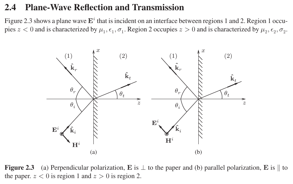
GA calculations

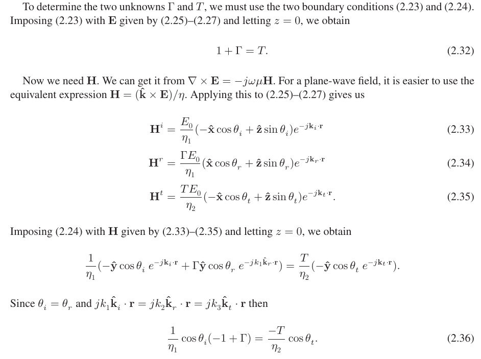
GA calculations

• If you are curious, have a look at the paper The Earth is not flat (Vanderbei, 2008), which implements a model using classical geometry to estimate the radius of the Earth.

• After having read and understood the paper, have a look at the same calculations done using GA: Sunset geometry (Merrill, 2016).

• Merrill’s approach requires to be proficient with GA calculation techniques, but it has two distinct advantages:

  1. No need to perform computations using sines and cosines;
  2. The relationships between angles come out naturally from the vectors, while in Vanderbei’s paper they need to be derived by hand.

Beyond GA

Two interesting sub-branches of Geometric Algebras are:

1. Projective geometric algebras: Generalizing the implicit equation for 3D planes ax + by + cz + d = 0, you can derive the concept of point and direction using a 4D space. (Homogeneous coordinates are born out of this.) See the YouTube Video A Swift Introduction to Projective Geometric Algebra;

2. Conformal geometric algebras: These are a further generalization of projective geometric algebras that can represent any conformal transformation (i.e., a transformation that preserves relative angles) in 3D space using a 5D (!) versor t, so that any of these transformations is just v' = t v t^{-1}.

Multivectors and Ray Tracing?

• Geometric algebra greatly simplifies the geometric equations needed in our course: scalars, vectors, planes, and volumes could be encoded by a single Multivector type, and transformations (rotations, translations, etc.) should be implemented only once: how wonderful!

• However, a multivector in ℝ³ requires 8 floating-point numbers to be stored: since ray tracers mostly use vectors, this is a waste (our Vec structure requires only 3 floating-point numbers).

• It is difficult (but not impossible) to implement efficient ray-tracing programs that use geometric algebra. A great reference is Geometric algebra for computer science (Dorst, 2007).

Further Reading (1/2)

• A swift introduction to geometric algebra: I took a few ideas and diagrams from here (YouTube video, about 40 minutes).

• Geometric Multiplication of Vectors (M. Josipović): it provides an intuitive idea of how geometric algebra works.

• Geometric Algebra for Physicists (C. Doran, A. Lasenby): comprehensive introduction to GA and its applications to physics: classical mechanics, special relativity, electromagnetism, quantum mechanics, Lagrangian formalism, gravitation, etc.

Further Reading (2/2)

• Understanding Geometric Algebra (K. Kanatani): more systematic than Josipović; it shows the link between homogeneous matrices and geometric algebra.

• Geometric algebra for computer science (Dorst, 2007): great introduction to projective geometric algebras. It contains a full implementation of a C++ library.

• A history of vector analysis (M. J. Crowe): this textbook describes the history of vector analysis, comparing the algebras of Hamilton, Grassmann/Clifford, and the vector system of Gibbs/Heavyside (which is the “classical” one, but it was born last).